
Cengage Financial Algebra 1st Edition Chapter 2 Exercise 2.5 Modeling a Business
Page 88 Problem 1 Answer
Given ; Fixed costs are$20,000.
cost of ear phone 5 $
The demand function is q=−200p+40,000
To find; Write the expense function in terms of q and determine a suitable viewing window for that function. Graph the expense function.

The expense function is E=5q+20000
Substitute for q to find the expense function in terms of priceq=−200p+40,000
E=5q+20000
E=5(−200p+40,000)+20000
E=−1000P+200000+20000
E=−1000P+220000
Read and Learn More Cengage Financial Algebra 1st Edition Answers
The horizontal axis represents price, and the vertical axis represents expense.
Both variables must be greater than 0,so the graph is in the first quadrant.
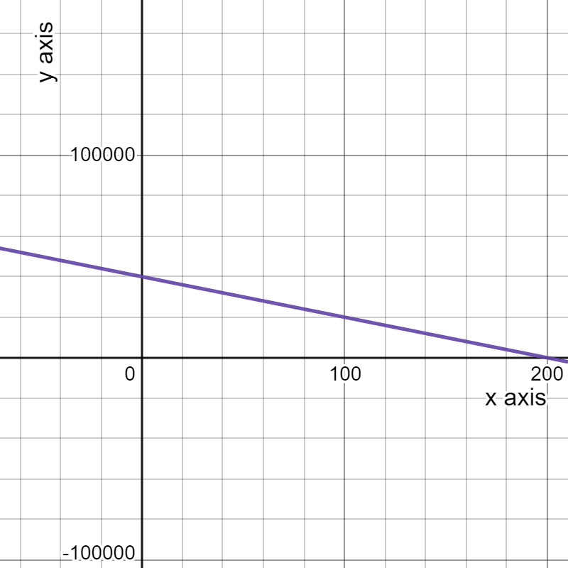
To determine a viewing window
find the points where the expense function intersects the vertical and horizontal axes.
Neither p nor E can be 0 because both a price of 0 and an expense of 0 would be meaningless in this situation.
But, you can use p=0 and E=0 to determine an appropriate viewing window
When p=0
E=−1000P+220000
E=−1000×0+220000
E=220000
or when E=0
E=−1000P+220000
0=−1000P+220000
1000P=220000
P=220000/1000
P=220
Hence we have express The expense function asE=5q+20000
Cengage Financial Algebra 1st Edition Chapter 2 Exercise 2.5 Modeling A Business Solutions
Cengage Financial Algebra 1st Edition Chapter 2 Exercise 2.5 Modeling a Business Page 88 Problem 2 Answer
Given:
The revenue equation for the Picasso Paints product is:
R= -500p2+30,000p
To find: The revenue if the price per item is set at
Solution: We will substitute the value in the equation
R= -500p2+30,000p
=-500(25)2+30,000(25)
=-312,500+750,000
=437,500
For the Picasso Paints product, if the price is $25 then the revenue will be$437,500
Page 89 Problem 3 Answer
Given that the prices $ 28, $40
To find the revenue
By using the example 3
From example 3 revenue equation is R=−500p2+30000p
for p=28
The revenue is
R=−500⋅(28)2
+30000⋅28
=−392000+840000
=448000
For p=40
The revenue is
R=−500⋅(40)2
+30000⋅40
=−800000+1200000
=400000
So, for p=28
we can get higher revenue
The revenue graph is

For p=28
we get higher revenue
The revenue graph is

Cengage Financial Algebra 1st Edition Chapter 2 Exercise 2.5 Modeling a Business Page 88 Problem 4 Answer
Given that prices are 7.50,61.00
To find why these prices are not in the best interest of the company
By using the example 3
From example 3 revenue equation is R=−500p2+30000p
The graph is
for p=7.50
The revenue is
R=−500⋅(7.5)2
+30000⋅7.5
=−28125+225000
=196875
For p=61.00
The revenue is
R=−500⋅(61)2
+30000⋅61
=−1860500+1830000
=−30500
For the prices 7.50,61.00, we get the lowest revenues.
So, these prices are not in the best interest of the company
The revenue graph is

Hence, proves that why those prices are not in the interest of the company
Page 90 Problem 5 Answer
Given that Money often costs too much
To find How might the quote apply to what you have learned
By using my own knowledge
The given quote is similar to another commonly used quote “Time is money”.
Thus if we want to earn money, then we will also have to sacrifice the time to get that money.
However, time is very costly for humans, as we only have a limited time that we get to spend on this planet and we never know when the “end” will be.
Thus money could then often cost too much if we have to sacrifice too much of our time to earn that money.
Cengage Financial Algebra Chapter 2 Exercise 2.5 Modeling A Business Answers
Cengage Financial Algebra 1st Edition Chapter 2 Exercise 2.5 Modeling a Business Page 90 Problem 6 Answer
Given that the demand function q=−1000p+8500
To find the expense equation
By using the given data
The costs are $1.00 per cup and $1,500.
Let E represent the total cost.
Let q be the demand (number of cups).
Then the total cost is the product of the costs per cup of $1.00 multiplied by the number of cups q, increased by the fixed costs of $1,500.
E=1.00q+1,500
The expense equation is E=1.00q+1,500
Page 90 Problem 7 Answer
Given that the demand function
q=−1000p+8500
To find the expense equation
By using the given data
From 2(a)
Expense equation E=1.00q+1500
given that q=−1000p+8500
By substituting q in E,
E=1,00(−1,000p+8,500)+1,500
=−1,000p+8,500+1,500
=−1,000p+10,000
The expense equation is E=−1,000p+10,000
Cengage Financial Algebra 1st Edition Chapter 2 Exercise 2.5 Modeling a Business Page 90 Problem 8 Answer
Given that the demand function
q=−1000p+8500
To find a viewing window on a graphing calculator for the expense function
By using the given data
From 2(b)
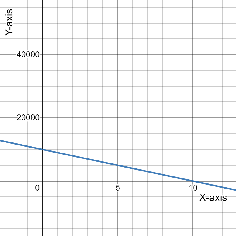
the expense function E=−1000p+10000
The graph for E is

The x-axis should contain values between 0 and 10 for p because the price and the expenses cannot be negative (and when the price is 10
the expenses become zero).
The y-axis should contain values between 0 and 10,000 because the price and the expenses cannot be negative (and the initial expenses are 10,000).
The graph for the expense equation is

The viewing window is
x: o to 10
y: 0 to 10000
Page 90 Problem 9 Answer
Given that the demand function
q=−1000p+8500
To draw the graph
By using the given data
From 2(b)
The expense equation is E=−1000p+10000
The graph is
The graph for the expense equation is

Page 90 Problem 10 Answer
Given that the demand function
q=−1000p+8500
To find the revenue function
By using the given data
The revenue function is the product between the demand function q and the price p.
R=pq
=p(−1,000p+8,500)
=−1,000p2+8,500p
The revenue function is R=−1,000p2+8,500p
Cengage Financial Algebra 1st Edition Chapter 2 Exercise 2.5 Modeling a Business Page 90 Problem 11 Answer
Given that the demand function
q=−1000p+8500
To f=draw revenue function
By using the given data
From 2(e)
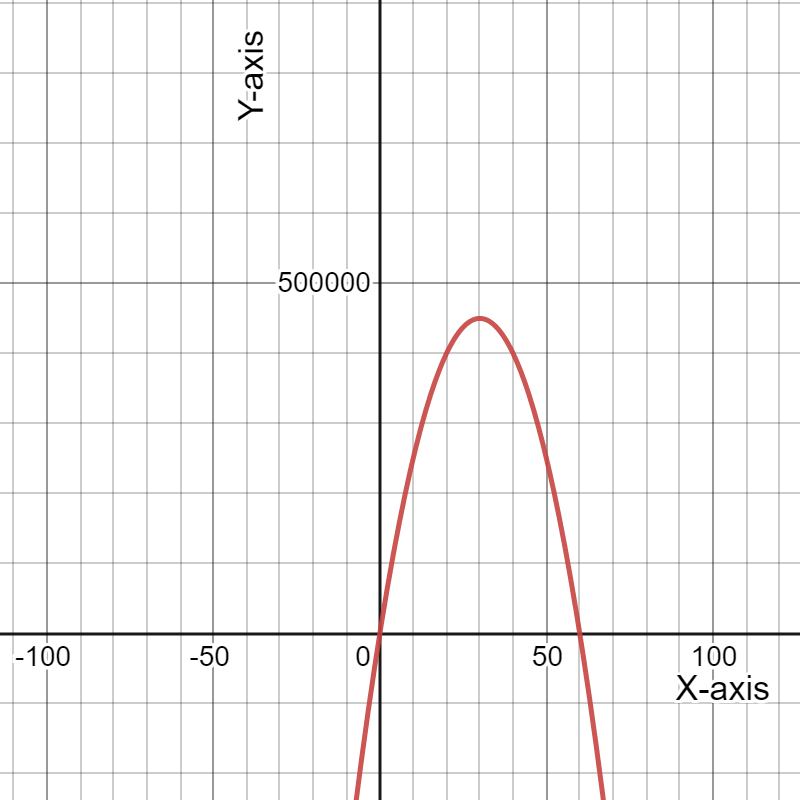
The revenue function is R=−1,000p2+8,500p
The graph is

Clearly, we can get maximum revenue of 18062.5 for 4.25
The graph for the revenue function is
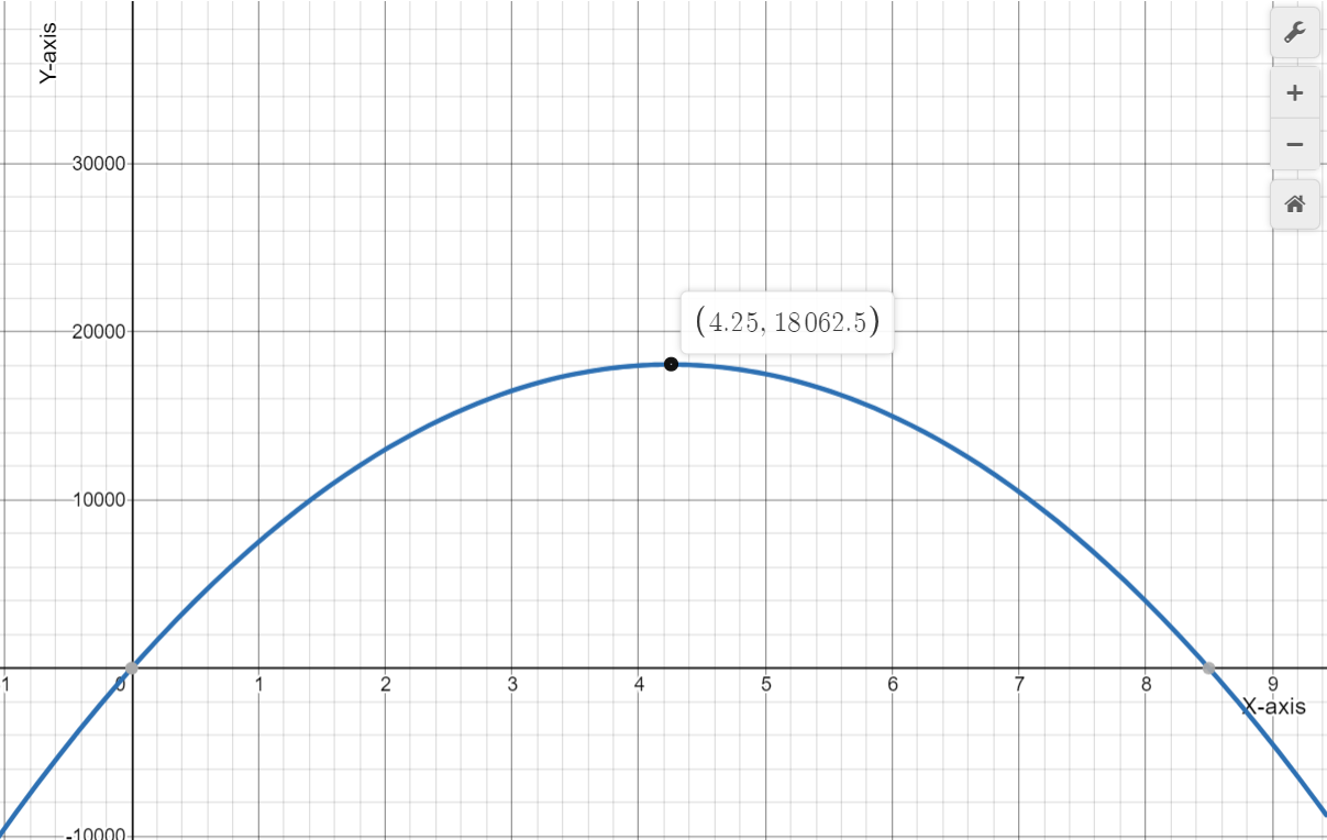
Maximum revenue: 18062.5 Price: 4.25
Page 90 Problem 12 Answer
Given that the demand function
q=−1000p+8500
To graph the revenue and expense functions on the same coordinate plane.
By using the given data
From 2(b)
Expense function E=−1000p+10000
From 2(e)
Revenue function R=−1,000p2+8,500p
The graph is
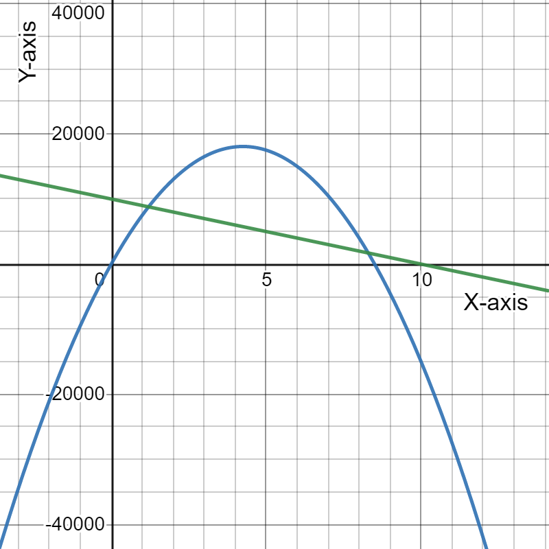
The intersection points are 1.2, 8.3
The graph is

The intersection points are 1.2, 8.3
Solutions For Cengage Financial Algebra Chapter 2 Exercise 2.5 Modeling A Business
Page 90 Problem 13 Answer
Given that the demand functionq=−500p+20000
To find the expense equation
By using the given data
The costs are $5.00 per box of 100 and a fixed cost of 40,000. Let q be the demand (number of boxes of 100).
E=5.00q+40,000
The expense equation is E=5.00q+40,000
Cengage Financial Algebra 1st Edition Chapter 2 Exercise 2.5 Modeling a Business Page 90 Problem 14 Answer
Given that the demand function
q=−500p+20000
To find the expense equation in terms of p
By using the given data
From 3(a)
The expense equation is E=5.00q+40000
given that q=−500p+20000
By substituting q in E, we get
E=5.00(−500p+20,000)+40,000
=−2,500p+100,000+40,000
=−2,500p+140,000
The expense equation is E=−2,500p+140,000
Page 90 Problem 15 Answer
Given that the demand function
q=−500p+20000
To find a viewing window on a graphing calculator for the expense function
By using the given data
From 3(b)
The expense equation is E=−2500p+140000
The graph is

The x-axis should contain values between 0 and 56 for p because the price and the expenses cannot be negative (and when the price is 56 the expenses become zero).
The y-axis should contain values between 0 and 140,000 because the price and the expenses cannot be negative (and the initial expenses are 140,000).
The graph for the expense equation is
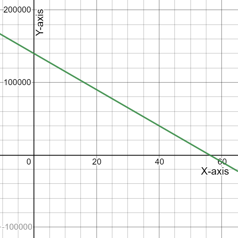
The viewing window is:
x-axis: 0 to 56
y-axis: 0 to 140000
Cengage Financial Algebra 1st Edition Chapter 2 Exercise 2.5 Modeling a Business Page 90 Problem 16 Answer
Given that the demand function
q=−500p+20000
To draw the graph
By using the given data
From 3(b)
The expense equation is E=−2500p+140000
The graph is

The graph for the expense equation is

Page 90 Problem 17 Answer
Given that the demand function
q=−500p+20000
To find the revenue function
By using the given data
Given that q=−500p+20000
The revenue function is
R=pq
=p(−500p+20,000)
=−500p2+20,000p
The revenue function is R=−500p2+20,000p
Page 90 Problem 18 Answer
Given that the demand function
q=−500p+20000
To graph the revenue function
By using the given data
From 3(e)
The revenue function is R=−500p2+20,000p
The graph is
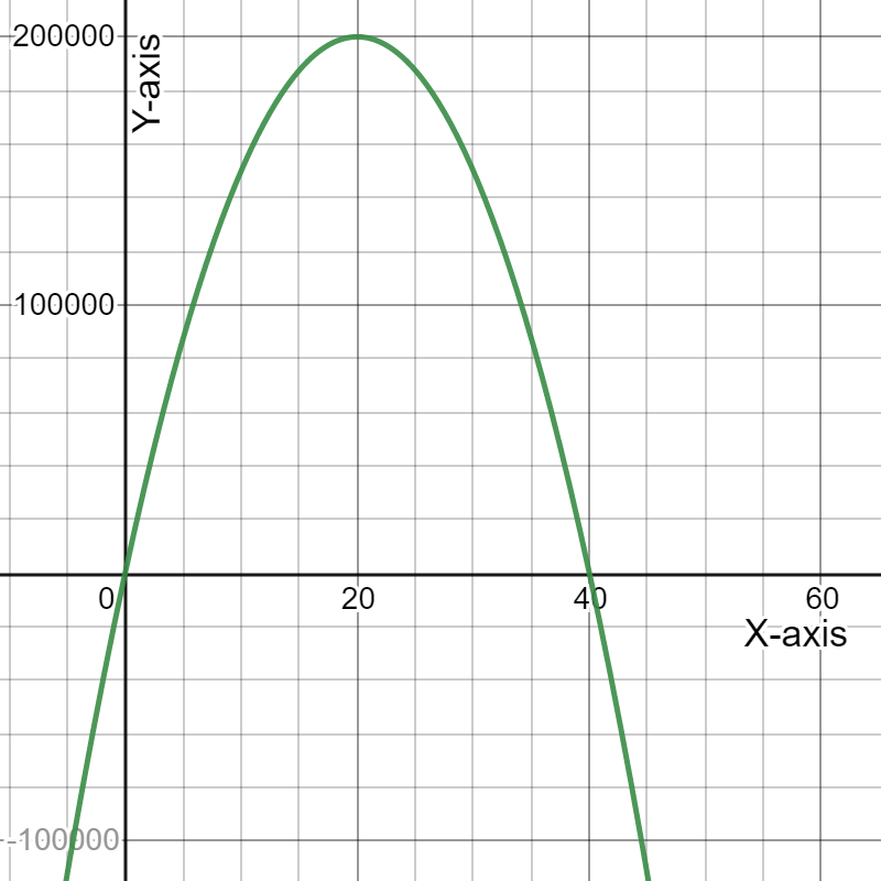
We get the maximum revenue of 200000
at p=20
The graph for revenue

The maximum revenue of 200000
at p=20
Cengage Financial Algebra Exercise 2.5 Modeling A Business Key
Cengage Financial Algebra 1st Edition Chapter 2 Exercise 2.5 Modeling a Business Page 90 Problem 19 Answer
Given that the demand function
q=−500p+20000
To graph the revenue and expense functions on the same coordinate plane
By using the given data
From 3(b)
The expense equation is E=−2500p+140000
From 3(e)
The revenue equation is R=−1000p2+8500p
The graph of expense and revenue equations on the same plane is

The intersection points are 7.5,37.5
The graph of expense and revenue equations on the same plane is
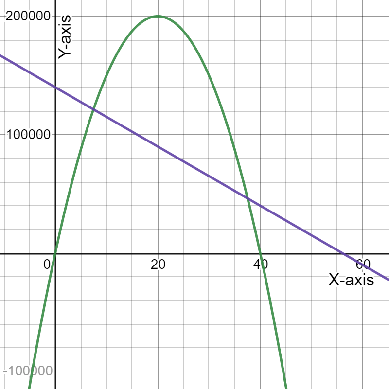
The intersection points are at prices 7.5, 37.5
Chapter 2 Solving Linear Inequalities
- Cengage Financial Algebra 1st Edition Chapter 2 Assessment Modeling a Business
- Cengage Financial Algebra 1st Edition Chapter 2 Exercise 2.1 Modeling a Business
- Cengage Financial Algebra 1st Edition Chapter 2 Exercise 2.2 Modeling a Business
- Cengage Financial Algebra 1st Edition Chapter 2 Exercise 2.3 Modeling a Business
- Cengage Financial Algebra 1st Edition Chapter 2 Exercise 2.4 Modeling a Business
- Cengage Financial Algebra 1st Edition Chapter 2 Exercise 2.6 Modeling a Business
- Cengage Financial Algebra 1st Edition Chapter 2 Exercise 2.7 Modeling a Business
- Cengage Financial Algebra 1st Edition Chapter 2 Exercise 2.8 Modeling a Business