Financial Algebra Cengage

Cengage Financial Algebra 1st Edition Chapter 2 Exercise 2.7 Modeling a Business

Page 99 Problem 1 Answer

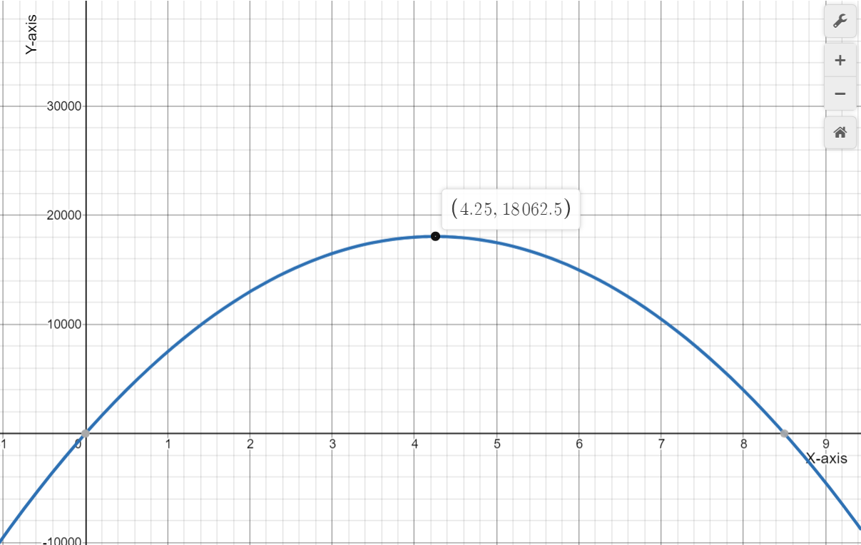
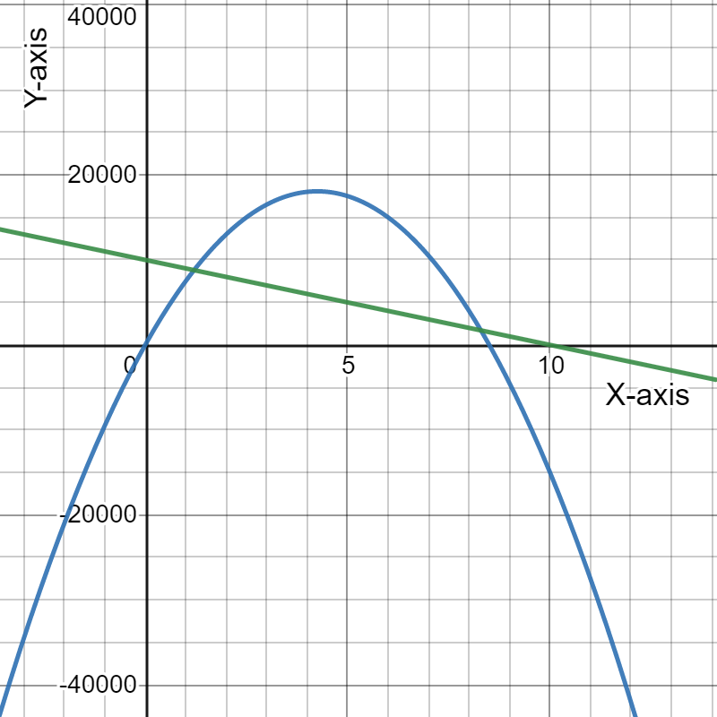
Given: The revenue and expense functions are R=-350p2+18,000p and E=−1,500p+199,000.

To find The profit equation. For doing so, we will use the fact that the difference between the revenue and total cost functions is the profit function.

We know that the difference between the revenue and total cost functions is the profit function.

P=R−E

=(−350p²+18,000p)−(−1,500p+199,000)

=−350p²+19500p−199000​

∴Our required profit equation isP=−350p2+19500p−199000.

Page 100 Problem 2 Answer

Given: Must maximum profit occur at the same price as the maximum revenue?

To find The explanation for the given.

We know that the profit equation is different from the revenue equation.

So, profit and revenue will have different parabolas with different points of maxima.

So, it is not necessary that maximum profit occurs at the same price as the maximum revenue.

No, it is not necessary that maximum profit occurs at the same price as the maximum revenue.

Page 101 Problem 3 Answer

Given: How might the quote apply to what has been outlined in this lesson?

To find: Summarize the lesson’s outline using a quote.

When you create a profit, your revenue exceeds your expenditures.

Read and Learn  More Cengage Financial Algebra 1st Edition Answers

When you lose money, your costs outnumber your earnings.

Because your income exceeds your costs, your expenses are not more than your revenue, implying that you cannot lose money if you earn a profit.

∴ You cannot lose money if you earn a profit.

Cengage Financial Algebra Chapter 2.7 Modeling A Business Guide

Cengage Financial Algebra 1st Edition Chapter 2 Exercise 2.7 Modeling a Business Page 101 Problem 4 Answer

Given:

To find The range of prices when the profit is made.

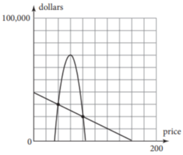
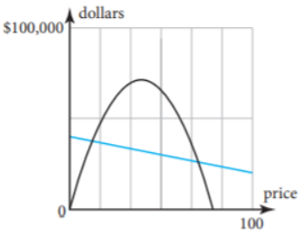
For doing so, we will refer to the fact that when the income exceeds the costs, the black curve rises over the blue line, indicating a profit.

When the income exceeds the costs, the black curve rises over the blue line, indicating a profit.

We can see that the horizontal axis is split into six regions between0 and 100, therefore the width between successive tick marks on the horizontal axis is:100/6≈16.67.

The initial crossing of the black curve and the blue line is about two-thirds of the way between the vertical axis and the first tick mark, which corresponds to11.11.

2/3⋅100/6

=100/9

≈11.11

The second crossing of the black curve and blue line occurs about one-third of the way between the fourth and fifth tickmarks, corresponding to72.22.

(4+1/3)⋅100/6

=650/9

≈72.22

When the price is generally between$11.11 and $72.22, we profit.

Page 101 Problem 5 Answer

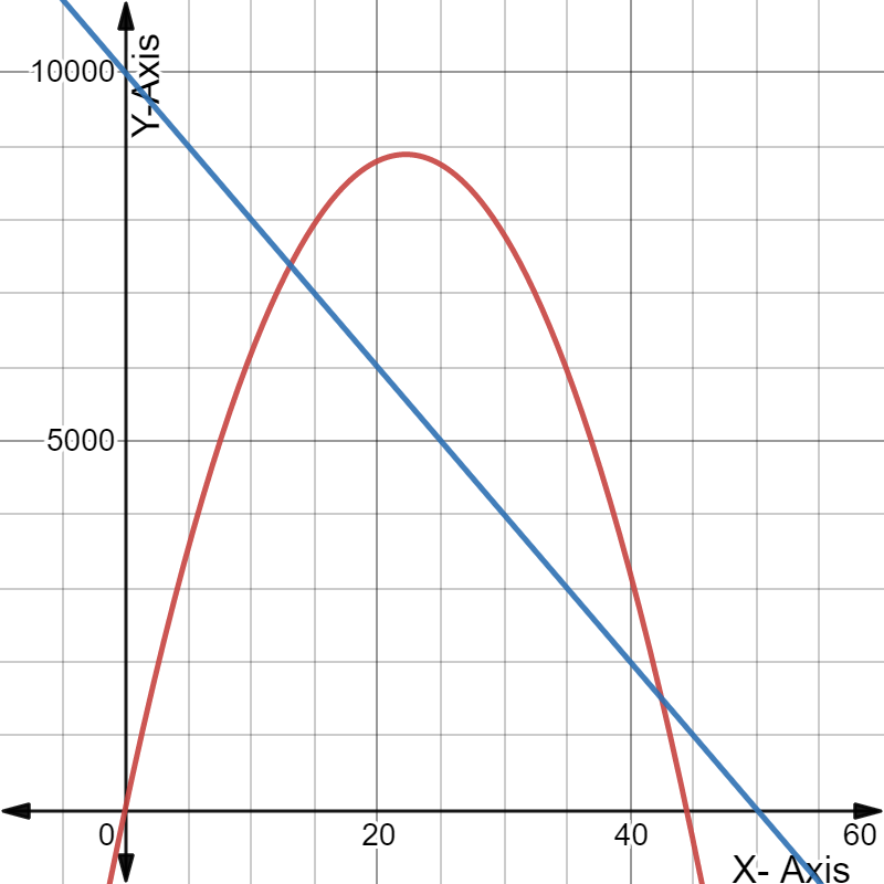
We have given a graph where the blue graph represents the expense function and the black graph represents the revenue function.

We have to describe the profit situation in terms of the expense and revenue functions.

We will use above information.

Here,We can see that between 0 and 100 on the horizontal axis is divided into 6 areas.

So, the width between the consecutive tick-marks on the horizontal axis is: 100/6

≈16.67

Now, The first intersection between the black curve and blue line is about one third between the vertical axis and the first tick-mark, which corresponds with roughly 11.11.

i.e.1/3⋅100/6

=50/9

≈5.56

The second intersection between the black curve and blue line is about two thirds between the fourth and fifth tick-mark, which corresponds with roughly 72.22

i.e.(4+2/3)⋅100/6

=700/9

≈77.78

Hence,

We make a profit when the price is roughly between $5.56 and $77.78.

Therefore, Price is roughly between $5.56 and $77.78

Cengage Financial Algebra 1st Edition Chapter 2 Exercise 2.7 Modeling a Business Page 101 Problem 6 Answer

Given : ​

E=−20,000p+90,000

R=−2,170p²+87,000p​

We have to write the profit function for the given expense and revenue functions.

We will use above information.

Here, We have, ​

E=−20,000p+90,000

R=−2,170p²+87,000p

So,P=−2,170p²+87,000p−(−20,000p+90,000)

​=−2,170p²+107,000p−90,000

​Therefore,

P=−2,170p²+107,000p−90,000

Page 101 Problem 7 Answer

Given : ​

E=−6,500p+300,000

R=−720p²+19,000p​

We have to write the profit function for the given expense and revenue functions.

We will use above information.

Here,We have,

E=−6,500p+300,000

R=−720p²+19,000p​

So, ​​P=−720p²+19,000p−(−6,500p+300,000)​

=−720p²+25,500p−300,000​

Therefore,

P=−720p²+25,500p−300,000

Cengage Financial Algebra 1st Edition Chapter 2 Exercise 2.7 Modeling a Business Page 101 Problem 8 Answer

Given : ​

E=−2,500p+80,000

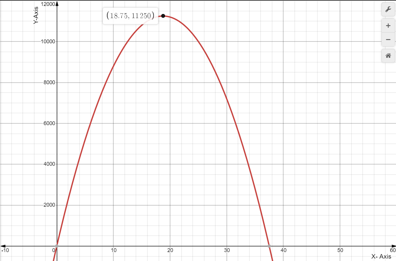
R=−330p²+9,000p​

We have to write the profit function for the given expense and revenue functions.

We will use above information.

Here, We have, ​

E=−2,500p+80,000

R=−330p²+9,000p​

so,P=−330p²+9,000p−(−2,500p+80,000)​

=−330p²+11,500p−80,000​

Therefore,

P=−330p²+11,500p−80,000

Page 101 Problem 9 Answer

Given : ​

E=−12,500p+78,000

R=−1,450p²+55,000p​

We have to write the profit function for the given expense and revenue functions.

We will use above information.

Here, We have, ​

E=−12,500p+78,000

R=−1,450p²+55,000p

So,P=−1,450p²+55,000p−(−12,500p+78,000)

​=−1,450p²+67,500p−78,000

​Therefore,

P=−1,450p²+67,500p−78,000

Financial Algebra 1st Edition Modeling A Business Exercise Solutions

Cengage Financial Algebra 1st Edition Chapter 2 Exercise 2.7 Modeling a Business Page 102 Problem 10 Answer

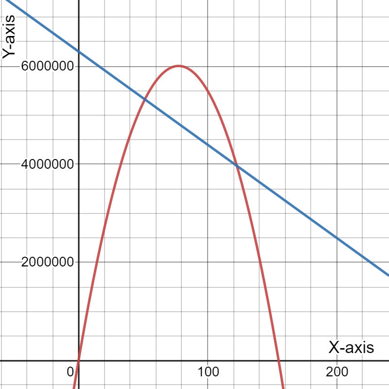
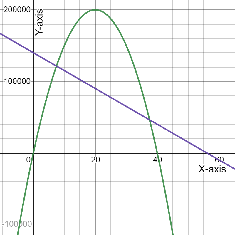
Given: The revenue (black) and expense (blue) functions.

We have to examine the revenue (black) and expense (blue) functions.

And also estimate the price at the maximum profit and explain our reasoning.

We will use above information.

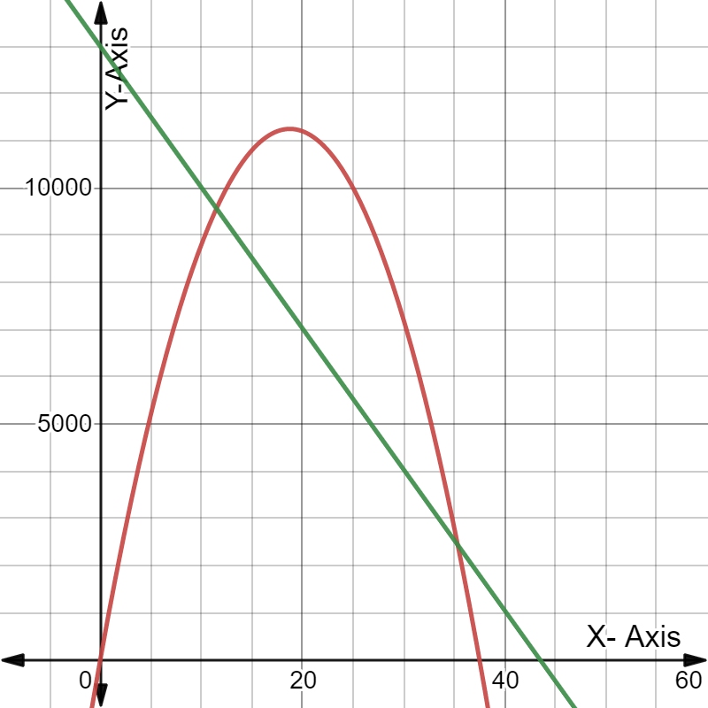
Here, As we know that, A profit is made when the revenue is larger than the expenses.

The maximum profit is then obtained when the difference between the revenue and expenses is largest.

The largest profit then appears to occur slightly to the right of the peak of the black curve.

Hence, The largest profit appears to occur at $25.00.

Therefore, The largest profit appears to occur at $25.00.

Page 102 Problem 11 Answer

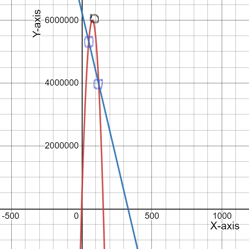
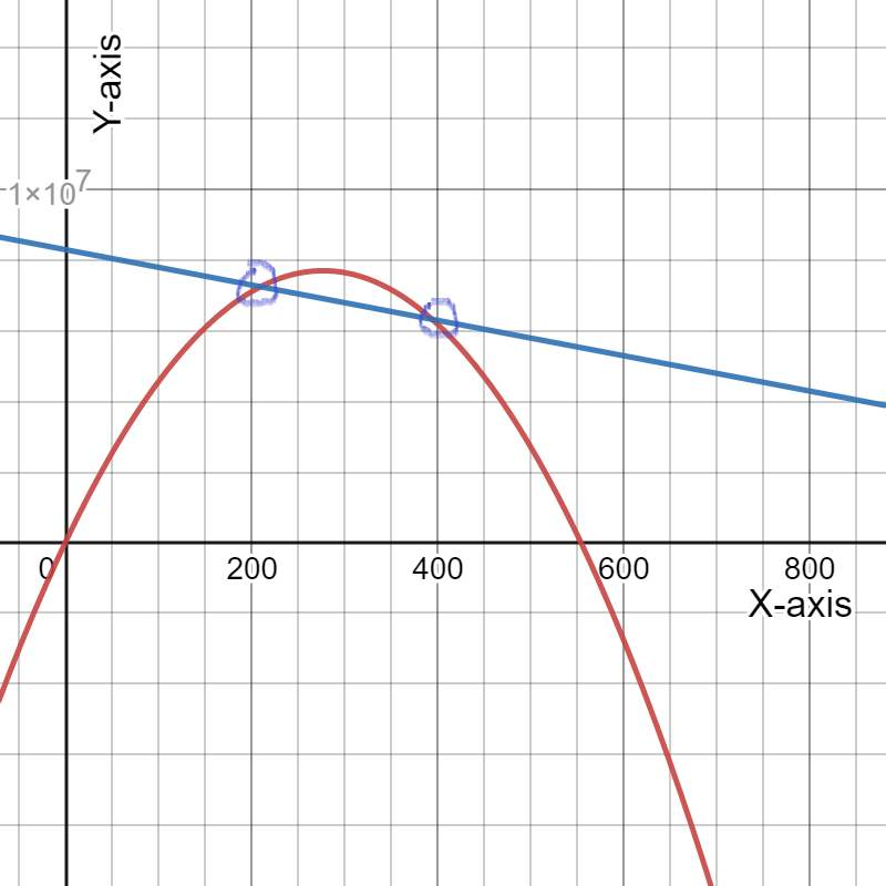
Given : Profit functions of Exercises 6−9 models .

We have to determine which profit function models a no profit situation.

We will use above information.

Here, We have, The profit function is the difference between the revenue function and the expense function.

P=−2,170p²+107,000p−90,000

P=−720p²+25,500p−300,000

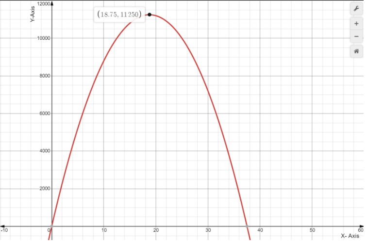
P=−330p²+11,500p−80,000

P=−1,450p²+67,500p−78,000

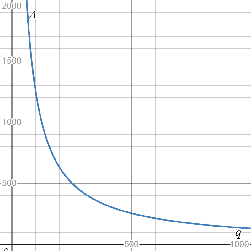
Now, the graph of all functions:

As the profit functions models a no profit situation if the profit is always negative (which indicates that we always make a loss and thus never make a profit).

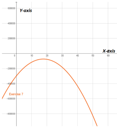
We see that the profit function of exercise 7 models a no profit situation, as the graph lies completely below the horizontal axis, which indicates that the profit is always negative.

Therefore,

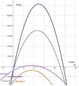
Problem 7 model is a no profit situation.

Cengage Financial Algebra 1st Edition Chapter 2 Exercise 2.7 Modeling a Business Page 102 Problem 12 Answer

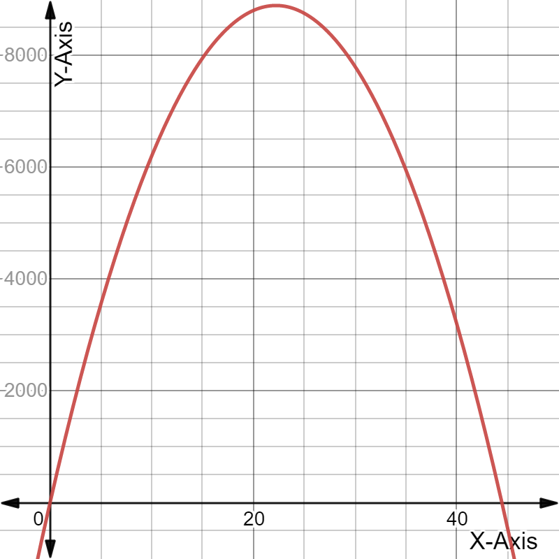
Given: Profit functions of Exercises 6−9 models.

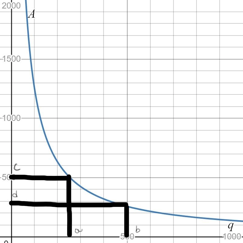
We have to show that how a profit function look like when no profit can be made.

We will use above information.

Here,The profit functions models a no profit situation if the profit is always negative (which indicates that we always make a loss and thus never make a profit).

As in part (a), we saw that the profit function of problem 7 models a no profit situation, as the graph lies completely below the horizontal axis, which indicates that the profit is always negative.

Thus a profit function lies completely below the horizontal axis when no profit can be made.

Therefore,

Page 102 Problem 13 Answer

Given : P=−400p²+12,400p−50,000

We have to determine the maximum profit and the price that would yield the maximum profit.

We will use above information.

Here,We have, ​​P=−400p²+12,400p−50,000,

a=−400​

b=12,400

c=−50,000​

As we know that the maximum value occurs on the axis of symmetry.

The x-intercept of the axis of symmetry is determined −b/2a=−12,400/2×−400

⇒15.5

So, at p=15.5 the profit will be maximum.

Now, The maximum profit ,​​P=−400(15.5)²+12,400(15.5)−50,000,

P=−96,100+192,200−50,000

​=46,100

​Therefore, The maximum profit is 46,100

Cengage Financial Algebra 1st Edition Chapter 2 Exercise 2.7 Modeling a Business Page 102 Problem 14 Answer

Given:P=−370p²+8,800p−25,000

We have to determine the maximum profit and the price that would yield the maximum profit.

We will use above information.

Here,

We have, ​​P=−370p²+8,800p−25,000

a=−370​

b=8,800

c=−25,000​

As we know that the maximum value occurs on the axis of symmetry.

The x-intercept of the axis of symmetry is determined −b/2a

=−8,800

2×−370

⇒11.89

So, at p=11.89 the profit will be maximum.

Now,The maximum profit ,​​P=−370(11.89)²+8,800(11.89)−25,000

P=−52,307.68+104,632−25,000

​=27,324.32

​Therefore,

The maximum profit is, P=27,324.32

Chapter 2 Exercise 2.7 Financial Algebra Cengage Walkthrough

Page 102 Problem 15 Answer

Given: P=−170p²+88,800p−55,000

To Determine the maximum profit and the price that would yield the maximum profit for each.

To determine the maximum profit algebraically, recall that the maximum value occurs on the axis of symmetry.

For the profit function given on left side The x – intercept of the axis of symmetry is determined −b/2a

P=−170p²+88,800p−55,000,a=−170,b=88,800, and c=−55,000.

​Calculate −b/2a

=−88,800/2×−170

=261.18

Hence at p=261.18, the profit will be maximum now to find maximum profit substitute this value of p

P=−170(261.18)²+88,800(261.18)−55,000,

P=−11,596,548.71+23,192,784−55,000=11,541,235.29

​At 261.18 the maximum proft would be 11,541,235.29.

Cengage Financial Algebra 1st Edition Chapter 2 Exercise 2.7 Modeling a Business Page 102 Problem 16 Answer

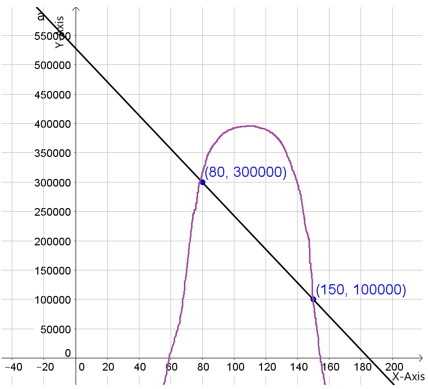
Given: The expense and revenue functions are

E=−1,850p+800,000 and R=−100p²+20,000p.

To Determine the profit function.

Using the formula P=R−E

we get

P=−100p²+20,000p−(−1,850p+800,000)

P=−100p²+21,850p−800,000

​Therefore profit function is  P=−100p²+21,850p−800,000

Page 102 Problem 17 Answer

Given: The expense and revenue functions are

E=−1,850p+800,000 and R=−100p²+20,000p.

To Determine the price, to the nearest cent, that yields the maximum profit.

To determine the maximum profit algebraically, recall that the maximum value occurs on the axis of symmetry. For the profit function given on left side The x – intercept of the axis

of symmetry is determined −b/2a

P=−100p²+21,850p−800,000

a=−100,b=21,850,c=−800,000

​Calculate −b/2a

=−21,850/2×−100

=109.25

Therefore the price, to the nearest cent, that yields the maximum profit at $109.25

Page 102 Problem 18 Answer

Given: The expense and revenue functions are

E=−1,850p+800,000 and R=−100p²+20,000p

Also From previous exercise we know that p=$109.25

To  Determine:  the maximum profit, to the nearest cent.

Hence at  p=109.25

The profit will be maximum now to find maximum profit substitute this value of p

P=−100(109.25)²+21,850(109.25)−800,000,

P=−1,193,556.25+2,387,112.5−800,000=393,556.25

​The maximum profit, to the nearest cent is $393,556.25

How To Solve Cengage Financial Algebra Chapter 2.7

Cengage Financial Algebra 1st Edition Chapter 2 Exercise 2.7 Modeling a Business Page 102 Problem 19 Answer

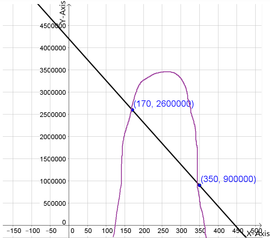
Given: The expense and revenue functions are  E=−250p+50,000 and R=−225p²+7,200p

To Determine the profit function.

p=−225p2+7,200p-(250p+50,000)

p=−225p2+7.450p−50.000

Therefore the profit function is P=−225p{2}+7.450p−50.000

Page 102 Problem 20 Answer

Given: expense and revenue functions are E=−250p+50,000 and R=−225p²+7,200p

To Determine: the price, to the nearest cent, that yields the maximum profit.

To determine the maximum profit algebraically, recall that the maximum value occurs on the axis of symmetry.

For the profit function given on left side The x – intercept of the axis of symmetry is determined −b/2a

P=−225p2+7,450p−50,000

a=−225,b=7,450,c=−50,000

Calculate −b/2a

=−7,450/2×−225

=16.56

Therefore the price, to the nearest cent, that yields the maximum profit is at $16.56

Page 102 Problem 21 Answer

Given : The expense and revenue functions are E=−250p+50,000 and R=−225p²+7,200p

Also we know that p=$16.56

To  Determine the maximum profit, to the nearest cent.

Hence at p=25.54 the profit will be maximum now to find maximum profit substitute this value of p

P=−225(16.56)²+7,450(16.56)−50,000

P=−61,702.56+123,372−50,000=11,669.44​

Therefore the maximum profit, to the nearest cent is at $11,669.44

Step-By-Step Guide To Financial Algebra Exercise 2.7

Chapter 2 Solving Linear Inequalities

• • Cengage Financial Algebra 1st Edition Chapter 2 Assessment Modeling a Business
  • Cengage Financial Algebra 1st Edition Chapter 2 Exercise 2.1 Modeling a Business
  • Cengage Financial Algebra 1st Edition Chapter 2 Exercise 2.2 Modeling a Business
  • Cengage Financial Algebra 1st Edition Chapter 2 Exercise 2.3 Modeling a Business
  • Cengage Financial Algebra 1st Edition Chapter 2 Exercise 2.4 Modeling a Business
  • Cengage Financial Algebra 1st Edition Chapter 2 Exercise 2.5 Modeling a Business
  • Cengage Financial Algebra 1st Edition Chapter 2 Exercise 2.6 Modeling a Business
  • Cengage Financial Algebra 1st Edition Chapter 2 Exercise 2.8 Modeling a Business

Cengage Financial Algebra 1st Edition Chapter 2 Exercise 2.6 Modeling a Business

Page 93 Problem 1 Answer

Given that there is an error when calculating the expense and revenue values

To find how we can improve the error By using basic knowledge

While we are using rounding off values, we can get some minute error in the revenue and expense values.

So, to improve on the error we have to use exact price values instead of the rounding values.

But it is somewhat difficult to calculate with the exact values manually.

Page 94 Problem 2 Answer

Given that ​E=−3500p+238000

R=−500p²+30000p​

To find a,b,c in cellsB11,B12,B13

By using basic calculations

Given that

E=−3500p+238000

R=−500p²+30000p

At breakeven point, The expense equals to revenue

−3500p+238000=−500p²+30000p

−500p²+33500p−238000=0

Read and Learn  More Cengage Financial Algebra 1st Edition Answers

​This equation is similar to the equation in cellB10

The a,b,c values are the values from the equation −500p²+33500p−238000=0

Cengage Financial Algebra 1st Edition Chapter 2 Exercise 2.6 Modeling A Business Solutions

Cengage Financial Algebra 1st Edition Chapter 2 Exercise 2.6 Modeling a Business Page 95 Problem 3 Answer

Given that Risk comes from not knowing what you’re doing

To find How might the quote apply to what you have learned

By using the own knowledge

If you don’t know what you are doing, then won’t know if you will make a profit or make a loss.

Moreover, you always won’t realize the extent of the possible loss and this could then provide a very large risk.

In practice, you will need to take into account your total expenses to determine the price of your items such that you won’t make any loss.

However, if you fail to do so, then you have a high risk of making a loss, as you didn’t check which prices will result in a profit for your company.

Page 95 Problem 4 Answer

Given that A supplier of school kits has determined that the combined fixed and variable expenses to market and sell G kits is W

To find breakeven point

By finding the price per item

The breakeven point is the price of one item

So, Breakeven point is W/G

Page 95 Problem 5 Answer

Given that A supplier of school kits has determined that the combined fixed and variable expenses to market and sell G kits is W

To find breakeven point

By finding the price per item

The cost per item is the total cost (which is 80%of W  ) divided by the number of items (2G).

The price per item is 80%×W

2GTo make breakeven the cost per item should equal the price (revenue) per item.

80%×W/2G

Cengage Financial Algebra 1st Edition Chapter 2 Exercise 2.6 Modeling a Business ​Page 95 Problem 6 Answer

Given that breakeven points are 80,150

To graph using the given data

By using the graph paper

Given that breakeven points are 80,150

At 80 the expense and revenue values are both 300000.

At 150, the expense and revenue values are both 100000.

The graph looks like

The graph is

Page 95 Problem 7 Answer

Given that breakeven points are 170, 350

To graph using the given data

By using the graph paper

Given that breakeven points are 170, 350

At 170 the expense and revenue values are both 2600000.

At 350 the expense and revenue values are both 900000.

The graph looks like

The graph is

Page 95 Problem 8 Answer

Given that expense function is E=−19,000p+6,300,000 and the revenue function is R=−1,000p²+155,000p

To Graph the expense and revenue functions. Label the maximum and minimum values for each axis. Circle the breakeven points.

By using the graphs

Given that

The expense function is E=−19,000p+6,300,000

The revenue function is R=−1,000p²+155,000p

The graph is

The breakeven points are blue circles and black circle is maximum value

The grap is

The breakeven points are blue circles and black circle is maximum value

Cengage Financial Algebra Chapter 2 Exercise 2.6 Modeling A Business Answers

Cengage Financial Algebra 1st Edition Chapter 2 Exercise 2.6 Modeling a Business Page 95 Problem 9 Answer

Given that: The expense function is E=−19,000p+6,300,000 And The revenue function is R=−1,000p²+155,000p

To find the prices at the breakeven points.

By using basic calculations

Given that

The expense function is E=−19,000p+6,300,000

The revenue function is R=−1,000p²+155,000p

At breakpoints, The revenue is equal to expense

−19,000p+6,300,000=−1,000p²+155,000p

1,000p²−174,000p+6,300,000=0

p=−174,000±√174,0002−4⋅1,000⋅6,300,000/2⋅1,000

=51.38 or 122.62

The graph is

​

The prices at breakeven points are 51.38 or 122.62

The graph is

Page 95 Problem 10 Answer

Given that:

The expense function is

E=−19,000p+6,300,000

The revenue function is

R=−1,000p²+155,000p

To find the revenue and expense amounts for each of the breakeven points.

By using basic calculations

From 7(b)

Breakeven points are 51.38, 122.62

At p=51.38,

The expense is ​​

E=−19,000⋅51.38+6,300,000

​=5,323,780

​So, the revenue=5,323,780

At p=122.62

The expense is

​​E=−19,000⋅122.62+6,300,000

​=3,970,220

​So, the revenue =3,970,220

At p=51.38, The expense and revenue is 5,323,780

At p=122.62, The expense and revenue is 3,970,220

Page 96 Exercise 1 Answer

Given that expense function is E=−5,000p+8,300,000 the revenue function is R=−100p{2}+55,500p

To Graph the expense and revenue functions. Circle the breakeven points.

By using the graphs

Given that expense function is

E=−5,000p+8,300,000 the revenue function is

R=−100p{2}+55,500p

Graph of the expense and revenue functions is

The graph is

Page 96 Exercise 2 Answer

Given that

expense function is

E=−5,000p+8,300,000 the revenue function is R=−100p{2} +55,500p

To find the prices at the breakeven points.

By using basic calculations

Given that expense function is

E=−5,000p+8,300,000 the revenue function is R=−100p{2}+55,500p

At breakeven point, The revenue is equal to expense

−5,000p+8,300,000=−100p²+55,500p

100p²−60,500p+8,300,000=0

p=60,500±√60,5002−4⋅100⋅8,300,000/2⋅100

=210.27 or 394.73​

The breakeven points are 210.3, 394.7

Solutions For Cengage Financial Algebra Chapter 2 Exercise 2.6 Modeling A Business

Cengage Financial Algebra 1st Edition Chapter 2 Exercise 2.6 Modeling a Business Page 96 Exercise 3 Answer

Given that expense function is

E=−5,000p+8,300,000 the revenue function is R=−100p{2}+55,500p

To find the revenue and expense amounts for each of the breakeven points

By using the graphs

Given that expense function is

E=−5,000p+8,300,000 the revenue function is R=−100p{2}+55,500p

From 8(b), The breakeven points are 210.27, 394.73

We know that At breakeven point, The revenue is equal to expense

At p=210.27,

The expense is E=−5,000⋅210.27+8,300,000

=7,248,646.67​

The revenue is 7,248,646.67

At p=394.73

The expense is E=−5,000⋅394.73+8,300,000 =6,326,353.33

​The revenue is 6,326,353.33

At p=210.27, The expense and revenue is 7,248,646.27

At p=394.73, The expense and revenue is 6,326,353.33

Page 96 Exercise 4 Answer

Given: The expense function isE=−200p+10,000 and the revenue function isR=−18p{2}+800p.

To find The price at which maximum revenue is reached and the maximum revenue.

For a parabola, the greatest revenue price is found along the axis of symmetry.

For a parabolay=ax{2}+b+c, the greatest revenue price is found along the axis of symmetryx=−b/2a.

We have​a=−32,

b=1200 and

c=0 ​in this situation because ofR=−18p{2}+800p.

p=−b/2a

=−800

2(−18)

=22.22.

As a result, the price at which the greatest revenue is achieved at$22.22.

Calculate the revenue that corresponds to the price of$22.22.

R=−18p²+800p

=−18(22.22)²+800(22.22)

≈$8888.89.

As a result, the maximum revenue is$8888.89.

The graph can be draw

∴ The maximum revenue of $ 8888.89 occurs at a price of $22.22.

Page 96 Exercise 5 Answer

Given: The expense and revenue functions exist.To do: Graph the given.For doing so, we will plot a graph.

The cost function is represented by a straight blue line, whereas the revenue function is represented by a red curve.

The cost function is represented by a straight blue line, whereas the revenue function is represented by a red curve.

Cengage Financial Algebra 1st Edition Chapter 2 Exercise 2.6 Modeling a Business Page 96 Exercise 6 Answer

Given: The expense function is E=−200p+10000 and the revenue function isR=−18p{2}+800p.

To find The prices at the breakeven points.For doing so, we will refer to the fact that at the breakeven point, the revenue and expenditure functions are equal.

At the breakeven point, the revenue and expenditure functions are equal.

−200p+10,000=−18p{2}+800p

⇒18p{2}

−1,000p+10,000=0.

Using the quadratic formula, find the solution.

​p=1,000±√1,000²−4⋅18⋅10,000 /2⋅18

=13.08 or 42.48

​The prices at the breakeven points are$13.08,$42.48.

Page 96 Exercise 7 Answer

Given: Breakeven prices are$13.08,$42.48.

To find The revenue and expense amount for each of the breakeven points.For doing so, we will refer to the fact that at the breakeven point, the revenue equals the expense.

We know that the breakeven prices are$13.08,$42.48.

Expenses corresponding these breakeven prices are​E=−200⋅13.08+10,000=7,384.17

E=−200⋅42.48+10,000

=1,504.72.

At the breakeven point, the revenue equals the expense. So​R=7,384.17,

R=1,504.72.

∴Our required amount of revenue and expenses are$7,384.17,$1,504.72.

Cengage Financial Algebra Exercise 2.6 Modeling A Business Key

Cengage Financial Algebra 1st Edition Chapter 2 Exercise 2.6 Modeling a Business Page 96 Exercise 8 Answer

Given: The expenses functionE=−300p+13000

and the revenue function isR=−32p{2}+1,200p.

To find: The price at which maximum revenue is reached and the maximum revenue.For a parabola, the greatest revenue price is found along the axis of symmetry.

For a parabolay=ax{2}+b+c, the greatest revenue price is found along the axis of symmetryx=−b/2a.

We have​a=−32,

b=1200 and

c=0 ​in this situation because ofR=−32p{2}+1,200p.

p=−b/2a

=−1200

2(−32)

=18.75.

As a result, the price at which the greatest revenue is achieved at$18.75.

A graph can be plotted as

∴The maximum revenue can be achieved at a price of$18.75.

Page 96 Exercise 9 Answer

Given: The maximum revenue can be achieved at a price of$18.75.

To find The maximum revenue.For doing so we will determine the revenue at a given price using the function provided.

Calculate the revenue that corresponds to the price of$18.75.

R=−18p²+800p

=−18(18.75)²+800(18.75)

≈$11,250.

As a result, the maximum revenue is$11,250.

The maximum revenue is$11,250.

Cengage Financial Algebra 1st Edition Chapter 2 Exercise 2.6 Modeling a Business Page 96 Exercise 10 Answer

Given: The expense and revenue functions exist.To do: Graph the given.For doing so, we will plot a graph.

The cost function is represented by a straight green line, whereas the revenue function is represented by a red curve.

The cost function is represented by a straight green line, whereas the revenue function is represented by a red curve.

Page 96 Exercise 11 Answer

Given: The expense functionE=−300p+13000p, and revenue function isR=−32p{2}+1,200p.

To find The prices at the breakeven points.

For doing so, we will refer to the fact that at the breakeven point, the revenue and expenditure functions are equal.

At the breakeven point, the revenue and expenditure functions are equal.

−300p+13,000=−32p{2}+1,200p

⇒32p{2}

−1,500p+13,000=0.

Using the quadratic formula, find the solution.​

p=1,500±√1,500²−4⋅32⋅13,000 /2⋅32

=11.48 or 35.40

∴The prices at the breakeven points are$11.48,$35.40.

Page 96 Exercise 12 Answer

Given: Breakeven prices are$11.48,$35.40.To find: The revenue and expense amount for each of the breakeven points.

For doing so, we will refer to the fact that at the breakeven point, the revenue equals the expense.

We know that the breakeven prices are$11.48,$35.40.

Expenses corresponding to these breakeven prices are​E=−300⋅11.48+13,000

=9,557.06

E=−300⋅35.40+13,000

=2,308.44.

At the breakeven point, the revenue equals the expense. So​R=9,557.06,

R=2,308.44.

Our required amount of revenue and expenses are$9,557.06,$2,308.44.

Cengage Financial Algebra 1st Edition Chapter 2 Exercise 2.6 Modeling a Business Page 96 Exercise 13 Answer

Given:

To find The price at which the maximum profit is reached.

The highest revenue yields the biggest profit; the revenue is determined by the parabola.

The highest point of the parabola is found on the third vertical line, which occurs at a cost of$60.

∴ The price at which the maximum profit is reached is$60.

Detailed Solutions For Cengage Financial Algebra Chapter 2 Exercise 2.6

Chapter 2 Solving Linear Inequalities

• • Cengage Financial Algebra 1st Edition Chapter 2 Assessment Modeling a Business
  • Cengage Financial Algebra 1st Edition Chapter 2 Exercise 2.1 Modeling a Business
  • Cengage Financial Algebra 1st Edition Chapter 2 Exercise 2.2 Modeling a Business
  • Cengage Financial Algebra 1st Edition Chapter 2 Exercise 2.3 Modeling a Business
  • Cengage Financial Algebra 1st Edition Chapter 2 Exercise 2.4 Modeling a Business
  • Cengage Financial Algebra 1st Edition Chapter 2 Exercise 2.5 Modeling a Business
  • Cengage Financial Algebra 1st Edition Chapter 2 Exercise 2.7 Modeling a Business
  • Cengage Financial Algebra 1st Edition Chapter 2 Exercise 2.8 Modeling a Business

Cengage Financial Algebra 1st Edition Chapter 2 Exercise 2.5 Modeling a Business

Page 88 Problem 1 Answer

Given ; Fixed costs are$20,000.

cost of ear phone 5 $

The demand function is q=−200p+40,000

To find; Write the expense function in terms of q and determine a suitable viewing window for that function. Graph the expense function.

The expense function is E=5q+20000

Substitute for q to find the expense function in terms of priceq=−200p+40,000

E=5q+20000

E=5(−200p+40,000)+20000

E=−1000P+200000+20000

E=−1000P+220000

Read and Learn  More Cengage Financial Algebra 1st Edition Answers

The horizontal axis represents price, and the vertical axis represents expense.

Both variables must be greater than 0,so the graph is in the first quadrant.

To determine a viewing window

find the points where the expense function intersects the vertical and horizontal axes.

Neither p nor E can be 0 because both a price of 0 and an expense of 0 would be meaningless in this situation.

But, you can use p=0 and E=0 to determine an appropriate viewing window

When p=0

E=−1000P+220000

E=−1000×0+220000

E=220000

​or when E=0

E=−1000P+220000

0=−1000P+220000

1000P=220000

P=220000/1000

P=220

​Hence we have express The expense function asE=5q+20000

Cengage Financial Algebra 1st Edition Chapter 2 Exercise 2.5 Modeling A Business Solutions

Cengage Financial Algebra 1st Edition Chapter 2 Exercise 2.5 Modeling a Business Page 88 Problem 2 Answer

Given:

The revenue equation for the Picasso Paints product is:

R= -500p2+30,000p

To find: The revenue if the price per item is set at

Solution: We will substitute the value in the equation

R= -500p²+30,000p

=-500(25)²+30,000(25)

=-312,500+750,000

=437,500

For the Picasso Paints product, if the price is $25 then the revenue will be$437,500

Page 89 Problem 3 Answer

Given that the prices $ 28, $40

To find the revenue

By using the example 3

From example 3 revenue equation is R=−500p²+30000p

for p=28

The revenue is

R=−500⋅(28)²

+30000⋅28

=−392000+840000

=448000

For p=40

The revenue is

R=−500⋅(40)²

+30000⋅40

=−800000+1200000

=400000

So, for p=28

we can get higher revenue

The revenue graph is

For p=28

we get higher revenue

The revenue graph is

Cengage Financial Algebra 1st Edition Chapter 2 Exercise 2.5 Modeling a Business Page 88 Problem 4 Answer

Given that prices are 7.50,61.00

To find why these prices are not in the best interest of the company

By using the example 3

From example 3 revenue equation is R=−500p²+30000p

The graph is

for p=7.50

The revenue is

R=−500⋅(7.5)²

+30000⋅7.5

=−28125+225000

=196875

For p=61.00

The revenue is

R=−500⋅(61)²

+30000⋅61

=−1860500+1830000

=−30500​

For the prices 7.50,61.00, we get the lowest revenues.

So, these prices are not in the best interest of the company

The revenue graph is

Hence, proves that why those prices are not in the interest of the company

Page 90 Problem 5 Answer

Given that Money often costs too much

To find How might the quote apply to what you have learned

By using my own knowledge

The given quote is similar to another commonly used quote “Time is money”.

Thus if we want to earn money, then we will also have to sacrifice the time to get that money.

However, time is very costly for humans, as we only have a limited time that we get to spend on this planet and we never know when the “end” will be.

Thus money could then often cost too much if we have to sacrifice too much of our time to earn that money.

Cengage Financial Algebra Chapter 2 Exercise 2.5 Modeling A Business Answers

Cengage Financial Algebra 1st Edition Chapter 2 Exercise 2.5 Modeling a Business Page 90 Problem 6 Answer

Given that the demand function q=−1000p+8500

To find the expense equation

By using the given data

The costs are $1.00  per cup and $1,500.

Let E represent the total cost.

Let q be the demand (number of cups).

Then the total cost is the product of the costs per cup of $1.00 multiplied by the number of cups q, increased by the fixed costs of $1,500.

E=1.00q+1,500

The expense equation is E=1.00q+1,500

Page 90 Problem 7 Answer

Given that the demand function

q=−1000p+8500

To find the expense equation

By using the given data

From 2(a)

Expense equation E=1.00q+1500

given that q=−1000p+8500

By substituting q in E,

​E=1,00(−1,000p+8,500)+1,500

=−1,000p+8,500+1,500

=−1,000p+10,000

​The expense equation is E=−1,000p+10,000

Cengage Financial Algebra 1st Edition Chapter 2 Exercise 2.5 Modeling a Business Page 90 Problem 8 Answer

Given that the demand function

q=−1000p+8500

To find a viewing window on a graphing calculator for the expense function

By using the given data

From 2(b)

the expense function E=−1000p+10000

The graph for E is

The x-axis should contain values between 0 and 10 for p because the price and the expenses cannot be negative (and when the price is 10

the expenses become zero).

The y-axis should contain values between 0 and 10,000 because the price and the expenses cannot be negative (and the initial expenses are 10,000).

The graph for the expense equation is

The viewing window is

x: o to 10

y: 0 to 10000

Page 90 Problem 9 Answer

Given that the demand function

q=−1000p+8500

To draw the graph

By using the given data

From 2(b)

The expense equation is E=−1000p+10000

The graph is

The graph for the expense equation is

Page 90 Problem 10 Answer

Given that the demand function

q=−1000p+8500

To find the revenue function

By using the given data

The revenue function is the product between the demand function q and the price p.

​​R=pq

​=p(−1,000p+8,500)

=−1,000p²+8,500p

​The revenue function is R=−1,000p²+8,500p

Cengage Financial Algebra 1st Edition Chapter 2 Exercise 2.5 Modeling a Business Page 90 Problem 11 Answer

Given that the demand function

q=−1000p+8500

To f=draw revenue function

By using the given data

From 2(e)

The revenue function is R=−1,000p²+8,500p

The graph is

Clearly, we can get maximum revenue of 18062.5 for 4.25

The graph for the revenue function is

Maximum revenue: 18062.5 Price: 4.25

Page 90 Problem 12 Answer

Given that the demand function

q=−1000p+8500

To graph the revenue and expense functions on the same coordinate plane.

By using the given data

From 2(b)

Expense function E=−1000p+10000

From 2(e)

Revenue function R=−1,000p²+8,500p

The graph is

The intersection points are 1.2, 8.3

The graph is

The intersection points are 1.2, 8.3

Solutions For Cengage Financial Algebra Chapter 2 Exercise 2.5 Modeling A Business

Page 90 Problem 13 Answer

Given that the demand functionq=−500p+20000

To find the expense equation

By using the given data

The costs are $5.00 per box of 100 and a fixed cost of  40,000. Let q be the demand (number of boxes of 100).

E=5.00q+40,000​

The expense equation is E=5.00q+40,000

Cengage Financial Algebra 1st Edition Chapter 2 Exercise 2.5 Modeling a Business Page 90 Problem 14 Answer

Given that the demand function

q=−500p+20000

To find the expense equation in terms of p

By using the given data

From 3(a)

The expense equation is E=5.00q+40000

given that q=−500p+20000

By substituting q in E, we get

​E=5.00(−500p+20,000)+40,000

=−2,500p+100,000+40,000

=−2,500p+140,000

​The expense equation is E=−2,500p+140,000

Page 90 Problem 15 Answer

Given that the demand function

q=−500p+20000

To find a viewing window on a graphing calculator for the expense function

By using the given data

From 3(b)

The expense equation is E=−2500p+140000

The graph is

The x-axis should contain values between 0 and 56 for p because the price and the expenses cannot be negative (and when the price is 56  the expenses become zero).

The y-axis should contain values between 0 and 140,000 because the price and the expenses cannot be negative (and the initial expenses are 140,000).

The graph for the expense equation is

The viewing window is:

x-axis: 0 to 56

y-axis: 0 to 140000

Cengage Financial Algebra 1st Edition Chapter 2 Exercise 2.5 Modeling a Business Page 90 Problem 16 Answer

Given that the demand function

q=−500p+20000

To draw the graph

By using the given data

From 3(b)

The expense equation is E=−2500p+140000

The graph is

The graph for the expense equation is

Page 90 Problem 17 Answer

Given that the demand function

q=−500p+20000

To find the revenue function

By using the given data

Given that q=−500p+20000

The revenue function is

R=pq

​=p(−500p+20,000)

=−500p²+20,000p

​The revenue function is R=−500p²+20,000p

Page 90 Problem 18 Answer

Given that the demand function

q=−500p+20000

To graph the revenue function

By using the given data

From 3(e)

The revenue function is R=−500p²+20,000p

The graph is

We get the maximum revenue of 200000

at p=20

The graph for revenue

The maximum revenue of 200000

at p=20

Cengage Financial Algebra Exercise 2.5 Modeling A Business Key

Cengage Financial Algebra 1st Edition Chapter 2 Exercise 2.5 Modeling a Business Page 90 Problem 19 Answer

Given that the demand function

q=−500p+20000

To graph the revenue and expense functions on the same coordinate plane

By using the given data

From 3(b)

The expense equation is E=−2500p+140000

From 3(e)

The revenue equation is R=−1000p²+8500p

The graph of expense and revenue equations on the same plane is

The intersection points are 7.5,37.5

The graph of expense and revenue equations on the same plane is

The intersection points are at prices 7.5, 37.5

Chapter 2 Solving Linear Inequalities

• • Cengage Financial Algebra 1st Edition Chapter 2 Assessment Modeling a Business
  • Cengage Financial Algebra 1st Edition Chapter 2 Exercise 2.1 Modeling a Business
  • Cengage Financial Algebra 1st Edition Chapter 2 Exercise 2.2 Modeling a Business
  • Cengage Financial Algebra 1st Edition Chapter 2 Exercise 2.3 Modeling a Business
  • Cengage Financial Algebra 1st Edition Chapter 2 Exercise 2.4 Modeling a Business
  • Cengage Financial Algebra 1st Edition Chapter 2 Exercise 2.6 Modeling a Business
  • Cengage Financial Algebra 1st Edition Chapter 2 Exercise 2.7 Modeling a Business
  • Cengage Financial Algebra 1st Edition Chapter 2 Exercise 2.8 Modeling a Business

Cengage Financial Algebra 1st Edition Chapter 2 Exercise 2.4 Modeling a Business

Page 81 Problem 1 Answer

Given that expense function for a certain product is E=3.40q+189,000

We have to express the average cost of producing q items algebraically.

Now we have the total cost for the q items as

E=3.40q+189,000

Now we have the average cost of producing as the total cost is divided by the total number of items that is

​3.40q+189,000/q

Average cost=3.40+189,000/q

Hence we have the average cost of producing q items algebraically is 340+189,000/q

Page 83 Problem 2 Answer

We have the  expense function, E=5.00q+60,000

And the revenue function, R=7.00q.

Now we have the breakeven point, set the revenue and expense equations equal to each other.

On equating we have

​E=R

5.00q+60,000=7.00q

2q=60,000

q=30,000

So we have the breakeven point as q=30,000

Hence we have the breakeven point as q=30,000

Read and Learn  More Cengage Financial Algebra 1st Edition Answers

Page 84 Problem 3 Answer

Given the statement as

An economist is an expert who will know tomorrow why the things he predicted yesterday didn’t happen today.

We have to interpret the quote.

If we predict about something yesterday then that predictions will be based on many variables and if any one of the variables changes slightly then it leads to different result today.

Therefore If we predict about something yesterday then that predictions will be based on many variables and if any one of the variables changes slightly then it leads to different result today.

Cengage Financial Algebra 1st Edition Chapter 2 Exercise 2.4 Modeling A Business Solutions

Cengage Financial Algebra 1st Edition Chapter 2 Exercise 2.4 Modeling a Business Page 84 Problem 4 Answer

Given that the Gidget Widget Corporation produces widgets.

The fixed expenses are $65,210 and the variable expenses are $4.22 per widget.

We have to express the expense function algebraically.

Let us assume that E be the total expense And let us assume q as the number of widgets

Now we know that the total expense as sum of expenses is the sum of fixed expenses plus the variable expenses we have

E=65210+4.22q

So we have the expense function algebraically as E=65210+4.22q

We have the expense function algebraically asE=65210+4.22q

Page 84 Problem 5 Answer

Given that A corporation produces mini-widgets.

The fixed expenses are $142,900 and the variable expenses are $1.24 per mini-widget.

We have to find how much does it cost to produce 1 mini-widget

Let us assume that E be the total expense

And Given that the number of widgets be 1

Now we know that the total expense as sum of expenses is the sum of fixed expenses plus the variable expenses we have

E=1.24×1+142,900

=142,901.24

​So we have obtained the cost to produce 1 mini-widget is $142,901.24

Hence the cost to produce 1 mini-widget is $142,901.24

Cengage Financial Algebra 1st Edition Chapter 2 Exercise 2.4 Modeling a Business Page 84 Problem 6 Answer

Given that A corporation produces mini-widgets.

The fixed expenses are $142,900 and the variable expenses are $1.24 per mini−widget.

We have to find how much does it cost to produce 20,000 mini-widget

Let us assume that E be the total expense

And Given that the number of widgets be 20000

Now we know that the total expense as sum of expenses is the sum of fixed expenses plus the variable expenses we have

E=1.24×20,000+142,900

=24,800+142,900

​=167,700

​So we have obtained the cost to produce 20000 mini-widget is $167,700

Hence the cost to produce 20000 mini-widget is $167,700

Page 84 Problem 7 Answer

Given that A corporation produces mini-widgets.

The fixed expenses are $142,900 and the variable expenses are $1.24 per mini−widget.

We have to express the expense function algebraically.

Let us assume that E be the total expense And let us assume q as the number of widgets

Now we know that the total expense as sum of expenses is the sum of fixed expenses plus the variable expenses we have

E=1.24q+142,900

So we have the expense function algebraically as E=1.24q+142,900

We have the expense function algebraically as E=1.24q+142,900

Cengage Financial Algebra Chapter 2 Exercise 2.4 Modeling A Business Answers

Page 84 Problem 8 Answer

From the above problem we have the expense function algebraically as E=1.24q+142,900

We have to find the slope of the expense function

As we have the expense function algebraically as E=1.24q+142,900

Now on comparing with the general form of the equation y=mx+c

We can say that the slope as 1.24

So we have the slope of the expense function as 1.24

Cengage Financial Algebra 1st Edition Chapter 2 Exercise 2.4 Modeling a Business Page 84 Problem 9 Answer

Given that A corporation produces mini-widgets.

The fixed expenses are $142,900 and the variable expenses are $1.24 per mini−widget.

We have to give the units that would be used.

As we have the slope as of form dy/dx

That is nothing but the units of y gets divided with the units of x

As we have the y as price so we have the unit as dollars  similarly we have x as number of mini widgets.

So we will have the unit of slope as dollars per mini -widgets.

Hence we have the units of slope as dollars per mini-widgets.

Page 84 Problem 10 Answer

We have the expense function for the Wonder Widget is E=4.14q+55,789

We have to find what is the fixed cost in the expense function

We have the expense function as E=4.14q+55,789

We will get the fixed cost in the expense function by substituing the value of number of mini-widgets as zero that is q=0

So we have the fixed cost as

​ Fixes cost =4.14(0)+55,789

=55,789

​So we have the fixed cost in the expense function as $55,789

Hence we have the fixed cost in the expense function as  $55,789

Page 84 Problem 11 Answer

In the above question they have given expense function of Wonder widgets

E=4.14q+55,789

We need to find the value cost producing for 500 woder widgets

Given

E=4.14q+55,789

The cost of producing q number of widgets is given by the equation replace q with 500 to find the cost of 500 widgets

E=4.14(500)+55,789

=2,070+55,789

=57859

​Hence the total value of cost producing 500 wonder widgets are 57859.

Cengage Financial Algebra 1st Edition Chapter 2 Exercise 2.4 Modeling a Business Page 84 Problem 12 Answer

In the above question they have given expense function of Wonder widgets

E=4.14q+55,789

We need to find the value cost producing for 500 woder widgets

Given

E=4.14q+55,789

We have found the cost of producing 500 widgets in previous part and it is 57859

Average cost for 500 widgets will be cost/500

Average cost =$57,859/500

=$115.718

≈$115.72

​Therefore average cost per producion 500 wonder widgets are 115.72

Page 84 Problem 13 Answer

In the above question they have given expense function of Wonder widgets

E=4.14q+55,789

We need to find the value cost producing for 500 woder widgets

Given

E=4.14q+55,789

The cost of producing q number of widgets is given by the equation  replace q with 600 to find the cost of 600 widgets

E=4.14(600)+55,789

=2,484+55,789

=58,273

​The total cost of producing 600 Wonder Widgets are 58,273.

Page 84 Problem 14 Answer

In the above question they have given expense function of Wonder widgets

E=4.14q+55,789

We need to find the value cost producing for 500 woder widgets

Given

E=4.14q+55,789

We have found the cost of producing 600 widgets in previous part and it is58273

Average cost for 600 widgets will be cost/ 600

Average cost​=$58,273/600

=$97.12166

≈$97.12

​The average cost per600

Wonder widgets is 97.12.

Solutions For Cengage Financial Algebra Chapter 2 Exercise 2.4 Modeling A Business

Cengage Financial Algebra 1st Edition Chapter 2 Exercise 2.4 Modeling a Business Page 84 Problem 15 Answer

In the above question they have given expense function of Wonder widgets

E=4.14q+55,789

We need to As the number of widgets increased from 500 to 600 did the average expense per widget increase or decrease

Given

E=4.14q+55,789

$115.72 Average cost per widget in case of 500

$97.12 Average cost per widget in case of 600

As 115.72 is greater than 97.12 it decreased

Therefore As the number of widgets increased from 500 to 600 the average expense per  widget decreased.

Page 84 Problem 16 Answer

In the above question they have given expense function of Wonder widgets

E=4.14q+55,789

We need to find the average cost per widgets of producing 10,000 wonder widgets

Given

E=4.14q+55,789

The cost of producing q number of widgets is given by the equation replace q with 10,000 to find the cost of 10,000 widgets

E=4.14(10,000)+55,789

=41,400+55,789

=97,189

​Average will be cost/10,000

Average cost​=$97,189/10,000

=$9.7189

≈$9.72

​The average cost per producing 10000 wonder widgets are 9.72.

Cengage Financial Algebra 1st Edition Chapter 2 Exercise 2.4 Modeling a Business Page 84 Exercise 1 Answer

Given​

q=−140p+9,000

E=2q+16,000

We need to express expense equation interms of p.

Given

q=−140p+9,000

E=2q+16,000

​Substitute the value of q in terms of p in equation for E

​E=2(−140p+9,000)

=−280p+18,000

​Expense function in term s of p is E=−280p+18,000

Page 84 Exercise 2 Answer

Given​

q=−140p+9,000

E=2q+16,000

​we need to find no. of widgets are demanded at a price of$ 10.00.

The demand function q is given by q= -140p+9,000

p is price

Now to find demand at price =$10 find q at p = 10

q=-140(10)+9,000

=7,600

Therefore 7,600 widgets are needed.

Page 84 Exercise 3 Answer

Given​

q=−140p+9,000

E=2q+16,000

we need to find cost to produce the number of widgetsfrom part b

Cost(Expense) function is given by

E=2q+16,000

q is number of widgets to be produced

Here q=7,600(from part b)

E=2(7,600)+16,000

=31,200

The total cost to produce 7600 widgets is 31200.

Cengage Financial Algebra 1st Edition Chapter 2 Exercise 2.4 Modeling a Business Page 84 Exercise 4 Answer

Given, expense equation as E=11.00q+76,000

Price of $20.00

We need to find items must be sold to reach the breakeven point to fin breakeven point revenue= Expense

Revenue=20q

Equate both and find a

20q=11q+76,000

3.9q=76,000

q=8,444.44 or 8,444

​8,444 items must be sold to reach the breakeven point.

Page 84 Exercise 5 Answer

Given​

Revenue =20q

Expense =11q+76,000

​We need to plot the graph and find the q value.

Ploting the graph of E and R

Hence q value is 8,444

The q value of exersice 9 and graph matches.

Page 84 Exercise 6 Answer

Given

E=4.98q+69,000

E′=4.55q+69,000

The expense equation was recently adjusted from E to E′  in response to the increase in gas prices

​We need find the incerase in the average cost per widget

Given

​E=4.98q+69,000

E′=4.55q+69,000

​Find the difference of new cost and previous cost

E−E′ =4.98q+69,000−(4.55q+69,000)

=0.43q

​So increase in average cost for 1 widget can be found by substituting q=1 in the difference

0.43(1)=0.43

0.43 is the increase in the average cost per widget.

Cengage Financial Algebra Exercise 2.4 Modeling A Business Key

Cengage Financial Algebra 1st Edition Chapter 2 Exercise 2.4 Modeling a Business Page 84 Exercise 7 Answer

Given

E=4.98q+69,000

E′=4.55q+69,000

The expense equation was recently adjusted from E to E′ in response to the increase in gas prices

Price p=8

We need to find breakeven point prior to the adjustment in the expense function.

To find breakeven point Revenue= expense

Revenue=8q

Expense=4.55q+69,000

equate both and find q

8q=4.55q+69,000

3.3.45q=69,000

q=20,000

E at q =20,000

E= 4.55(20,000)+69,000

=160,000

20,000 items are sold at breakeven point at the cost 160,000

Page 84 Exercise 8 Answer

Given

E=4.98q+69,000

E′=4.55q+69,000

The expense equation was recently adjusted from E to E′  in response to the increase in gas prices

​Price p=8.5

We need to find breakeven point after the adjustment in the expense function

To find breakeven point Revenue= expense

Revenue =8.5q

Expense =4.98q+69,000​

Equate both and find q

8.5q=4.98q+69,000

3.3.52q=69,000

q=19,602.27 or 19,602

​E at q=19,602

E=4.98(19,602)+69,000

=166,617.96 or 166,618​

items are sold at breakeven point at the cost166,618 .

Page 84 Exercise 9 Answer

In the above question they have given a graph We need to observe the graph and answer the question

” What is the breakeven point?”

Answer:-

Breakeven point is the point at which revenue = expense and this can be seen that point of intersection of both  lines is (A,W)

​The break even point is from (A,W).

Page 84 Exercise 10 Answer

In the above question they have given a graph

We need to observe the graph and answer the question

If quantity C is sold and C<A, is there a profit or a loss? Explain.

Answer:-

Drop a vertical line at q<A

then it is visible that revenue is less than expense and hence we can say there will be loss

Hence there will be loss.

Cengage Financial Algebra 1st Edition Chapter 2 Exercise 2.4 Modeling a Business Page 84 Exercise 11 Answer

In the above question they have given a graph

We need to observe the graph and answer the question

If quantity D is sold and D>A, is there a profit or a loss? Explain.

Answer:-

Drop a vertical line at q>A then it is visible that revenue is higher than expense and hence we can say there will be profit.

Hence there will be a profit.

Page 84 Exercise 12 Answer

In the above question they have given a graph

We need to observe the graph and answer the question​

The y−intercept of the expense function is Z.

Interpret what the company is doing if it operates at the point (0,Z).

Answer:-

If company is operating at(0,Z) that means company is not producing any product but still has to pay Z

dollars for the fixed expenses and yes company will be definitely in loss of Z dollars.

Hence the selling no goods but paying Z dollars for fixed expenses.

Page 85 Exercise 13 Answer

Given

E=6.21q+125,000

p=19.95

we need to represent the average expence A for one nokee algebraically.

Given

E for q number of goods is E=6.21q+125,000

Average expense if given by expense for q number of goods divided by q

E=6.21q+125,000/q.

Hence Average expence A for one nokee algebrically is E=6.21q+125,000/q.

Page 85 Exercise 14 Answer

Given

E=6.21q+125,000

p=19.95

we need to represent graph the average expense function.

Plotting the graph​

Set the range of x 0 to 1000

range of y 0 to 2000 and the value of y=6.21+(125,000/x)​

Hence the graph is plotted

Detailed Solutions For Cengage Financial Algebra Chapter 2 Exercise 2.4

Cengage Financial Algebra 1st Edition Chapter 2 Exercise 2.4 Modeling a Business Page 85 Exercise 15 Answer

Given

E=6.21q+125,000

p=19.95

we need to verify whether the average expense is linear or not.

By observing the graph

As seen in 13 b  the graph of average expense is not linear.

The average expense function is not linear.

Page 85 Exercise 16 Answer

Given

E=6.21q+125,000

p=19.95

we need to find whether the expence function is increasing or decreasing as q increasing.

Hence verage expense function increasing or decreasing as q increases.

Page 85 Exercise 17 Answer

Given

E=6.21q+125,000

p=19.95

if only one Nokee is produced we need to find the average cost per nokee

E for q number of goods is E=6.21q+125,000

Average expense if given by expense for q number of goods divided by q

E=6.21q+125,000/q

For 1 put q=1

6.21+125,000/1

=125,006.21

If only one Nokee is produced, what is the average cost per Nokee125,006.21.

Cengage Financial Algebra 1st Edition Chapter 2 Exercise 2.4 Modeling a Business Page 85 Exercise 18 Answer

Given

E=6.21q+125,000

p=19.95

if 100,000 Nokee is produced we need to find the average cost per nokee

E for q number of goods is E=6.21q+125,000

Average expense if given by expense for q number of goods divided by q

E=6.21q+125,000/q

For 100,000 put q=100,000

6.21(100,000+125,000

100,000

=7.46

If 100,000 Nokees are produced, then the average cost per Nokee 7.46

Page 85 Exercise 19 Answer

In the above question they have given that Lorne has determined the fixed cost of producing his new invention is N dollars.

Variable cost is $ 10.75

We need to find average cost per item.

Remember ,fixed expenses do not depend on the quality produced.

Thus, regradless of how big ‘W’ is, the fixed cost would still be N.

First find the total cost of producing W items:

=$10.75W+N

Divide by W to find average per item:

=$10.75W+N/W

=$10.75W/W+N/W

=$10.75+n/w

Hence the average cost per producing W item is $10.75+N/W.

Practice Problems For Cengage Financial Algebra Exercise 2.4 Modeling A Business

Chapter 2 Solving Linear Inequalities

• • Cengage Financial Algebra 1st Edition Chapter 2 Assessment Modeling a Business
  • Cengage Financial Algebra 1st Edition Chapter 2 Exercise 2.1 Modeling a Business
  • Cengage Financial Algebra 1st Edition Chapter 2 Exercise 2.2 Modeling a Business
  • Cengage Financial Algebra 1st Edition Chapter 2 Exercise 2.3 Modeling a Business
  • Cengage Financial Algebra 1st Edition Chapter 2 Exercise 2.5 Modeling a Business
  • Cengage Financial Algebra 1st Edition Chapter 2 Exercise 2.6 Modeling a Business
  • Cengage Financial Algebra 1st Edition Chapter 2 Exercise 2.7 Modeling a Business
  • Cengage Financial Algebra 1st Edition Chapter 2 Exercise 2.8 Modeling a Business

Cengage Financial Algebra 1st Edition Chapter 2 Exercise 2.3 Modeling a Business

Page 76 Problem 1 Answer

Given: Wholesale Price=x dollars

Retail Price=y dollars

To find: The markup amount

Solution:Wholesale price+Markup=Retail Price

x+Markup=y

Markup=y−x

The wholesale price of an item is x dollars and the retail price is y dollars, then the markup is y−x dollars

Page 77 Problem 2 Answer

Given: A banner company sells 5-foot banners to retailers for x dollars. The St. James Sign Shop marks them up90%

To find: Express the retail price at the St. James store

Solution: We will find the value of the markupThen find the retail price

Markup=90%of wholesale price

=90/100×x

=0.9x

Read and Learn  More Cengage Financial Algebra 1st Edition Answers

Retail price=Wholesale price+Markup

=x+0.90x

=1.90x

A banner company sells 5 -foot banners to retailers for x dollars and the St. James Sign Shop marks them up90%, then the retail price will be1.90x

Cengage Financial Algebra 1st Edition Chapter 2 Exercise 2.3 Modeling A Business Solutions

Cengage Financial Algebra 1st Edition Chapter 2 Exercise 2.3 Modeling a Business Page 77 Problem 3 Answer

If a widget has a low price, many people may want it and will be able to afford it, so a large quantity may be sold.If it has a high price, fewer widgets will be sold.

As the price increases, demand (the quantity consumers want) is likely to decrease, and as price decreases, demand increases.

The graph of the demand function has a negative slope. However, its curvature varies.

The demand function has a negative slope because as the price of a product increases the demand for the product will decrease.

Page 78 Problem 4 Answer

Here, we have to find the store’s markup. It’s given that an automobile GPS system is sold to stores at a wholesale price of $97

A popular store sells them for $179.99

Markup= Retail price−Wholesale price

=   $179.99−$97=$82.99

So, the store’s markup is$82.99

Page 78 Problem 5 Answer

Here, we have to find the retail price of the CD rack. It’s given that a CD storage rack is sold to stores at a wholesale price of $18

Retail price=Markup+Wholesale price

=$13+$18=$82.99

So, the retail price of the CD rack is $82.99

Page 79 Problem 6 Answer

Here, we have to find the equation of the linear regression line.

Enter the ordered pairs(p is wholesale price and y is quantity demanded in hundreds) into your calculator.

Then use the statistics menu to calculate the linear regression equation.

The equation is of the form y=mx+b,where m is the slope and b is the y intercept.

Rounding the slope and y intercept to the nearest hundredth, the equation of the regression line is −136.08p+2,535.79

So, the equation of the linear regression line is q=−136.08p+2,535.79

Page 79 Problem 7 Answer

Here, we have to give the slope of the regression line and interpret the slope as a rate.

As the line is q=−136.08p+2,535.79

Comparing it with y=mx+c,where m is slope,  q=mx+c=−136.08p+2,535.79,gives m=−136.08

The slope is −136.08.As a rate, the slope is expressed as garbage cans per dollar.

For each dollar increase in price, about 136 less garbage cans are demanded.

Page 79 Problem 8 Answer

Here, we have to find the correlation coefficient and interpret it.

Use a graphing calculator to find the correlation coefficient. Round r to the nearest hundredth r=−0.99.

As magnitude of r>0.75 hence strong correlation.

So, the  correlation coefficient is r=−0.99, there is a strong negative correlation.

Page 79 Problem 9 Answer

Here, we have to find how many garbage cans would be demanded at a wholesale price of $18.00.

For demand of garbage bans of downloads put p=18

(do not forget that unit of q was in hundred)

q=−136.08×18+2,535.79

y=−2,449.44+2,535.79

86.35≈86

​So, the garbage cans would be demanded at a wholesale price of $18.00 Is 86 hundred.

Cengage Financial Algebra Chapter 2 Exercise 2.3 Modeling A Business Answers

Cengage Financial Algebra 1st Edition Chapter 2 Exercise 2.3 Modeling a Business Page 79 Problem 10 Answer

Here, we have to determine whether our answer to part d is an example of extrapolation or interpolation and we have to explain.

In previous question the value of price was $18 which is out of the domain.

So, the answer to part d is an example of extrapolation,$18.00 is not in the domain.

Page 79 Problem 11 Answer

Here, we have to find how much money would the company receive from the garbage can sales. It’s given that

So, the money would the company receive from the garbage can sales is $154,800

Page 79 Exercise 1 Answer

Given that company that produces widgets has found its demand function to be q=−1,500p+90,000

For each dollar increase in the wholesale price we have to find how many fewer widgets are demanded

Now we have given the demand function as q=−1,500p+90,000

Now on  substituing value of p as p+1

q=−1,500(p+1)+90,000

=−1,500p−90,000−1,500

=q−1500​

Therefore we can say that 1500 widgets were demanded for each dollar increase in the wholesale price.

Hence the number of widgets demanded for each dollar increase in the wholesale price is 1500

Page 79 Exercise 2 Answer

Given that company that produces widgets has found its demand function to be q=−1,500p+90,000

For each dollar increase in the wholesale price we have to find how many fewer widgets are demanded

We have to find how  many widgets would be demanded at a price of $20

We have given the demand equation as q=−1,500p+90,000

Now we have

q=−1,500×20+90,000

=−30,000+90,000

=60,000​

Therefore the number of widgets demanded at a price of $20 is 60,000

Hence the number of widgets demanded at a price of $20 is 60,000.

Given that company that produces widgets has found its demand function to be q=−1,500p+90,000

For each dollar increase in the wholesale price we have to find how many fewer widgets are demanded

We have to find how many widgets would be demanded at a price of $21

We have given the demand equation as q=−1,500p+90,000

Now we have

q=−1,500×21+90,000

=−31,500+90,000

=58,500

​Therefore the number of widgets demanded at a price of $21 is 58,500

Hence the number of widgets demanded at a price of $21 is58,500

Solutions For Cengage Financial Algebra Chapter 2 Exercise 2.3 Modeling A Business

Cengage Financial Algebra 1st Edition Chapter 2 Exercise 2.3 Modeling a Business Page 79 Exercise 4 Answer

Given that company that produces widgets has found its demand function to be q=−1,500p+90,000

For each dollar increase in the wholesale price we have to find how many fewer widgets are demanded

We have to find what is the difference in quantity demanded caused by the $1 increase in wholesale price.

Now we have given the demand function as q=−1,500p+90,000

Now on  substituting value of p as p+1

​q=−1,500(p+1)+90,000

=−1,500p−90,000−1,500

=q−1500

q−q′

=1500​

Therefore the difference in quantity demanded caused by $1 increase in wholesale price is 1500

Hence  the difference in quantity demanded caused by $1 increase in wholesale price is 1500

Page 79 Exercise 5 Answer

Given that company that produces widgets has found its demand function to be q=−1,500p+90,000

For each dollar increase in the wholesale price we have to find how many fewer widgets are demanded

We have to find how many widgets would be demanded at a price of $22.50

We have given the demand equation as q=−1,500p+90,000

Now we have

q=-1,500×22.5+90,000

=-33,750+90,000

=56,250

Therefore the number of widgets demanded at a price of $22.5 is 56,250

Hence the number of widgets demanded at a price of $22.5 is 56,250

Cengage Financial Algebra 1st Edition Chapter 2 Exercise 2.3 Modeling a Business Page 79 Exercise 6 Answer

Given that company that produces widgets has found its demand function to be q=−1,500p+90,000

For each dollar increase in the wholesale price we have to find how many fewer widgets are demanded

We have to find how much will all of the widgets cost the store to purchase at a price of $

Now we have the Number of widgets as

q=−1,500×22.5+90,000

=−33,750+90,000

=56,250

​Now we have the cost as  the product of price to the number of widegets that is

cost price=$22.50×56,250

=$1,265,625

​So we have the cost to store all the widgets purchased at a price of $22.5 is $1,265,625

Hence we have the cost to store all the widgets purchased at a price of $22.5 is $1,265,625

Page 79 Exercise 7 Answer

Given that company that produces widgets has found its demand function to be q=−1,500p+90,000

store marks up the widgets that cost $22.50 at a rate of 50%,

We havr to to find the retail price of each widget.

Now we have the markup as the product of the cost with markup rate that is

Markup = $22.5×50%

​=$22.5×0.5

=$11.25

​Now we have the Retail price as the sum of markup to the wholesale price that is

Retail price =$22.5+$11.25

​=$33.75​

So we have the retail price as $33.75

Hence we have the retail price as $33.75

Cengage Financial Algebra Exercise 2.3 Modeling A Business Key

Chapter 2 Solving Linear Inequalities

• • Cengage Financial Algebra 1st Edition Chapter 2 Assessment Modeling a Business
  • Cengage Financial Algebra 1st Edition Chapter 2 Exercise 2.1 Modeling a Business
  • Cengage Financial Algebra 1st Edition Chapter 2 Exercise 2.2 Modeling a Business
  • Cengage Financial Algebra 1st Edition Chapter 2 Exercise 2.4 Modeling a Business
  • Cengage Financial Algebra 1st Edition Chapter 2 Exercise 2.5 Modeling a Business
  • Cengage Financial Algebra 1st Edition Chapter 2 Exercise 2.6 Modeling a Business
  • Cengage Financial Algebra 1st Edition Chapter 2 Exercise 2.7 Modeling a Business
  • Cengage Financial Algebra 1st Edition Chapter 2 Exercise 2.8 Modeling a Business

Cengage Financial Algebra 1st Edition Chapter 1 Exercise 1.1 The Stock Market

Page 6 Problem 1 Answer

Given: Jillian owns60%of the stock in a private catering corporationThere are1,200shares in the entire corporation

To find: The number of shares owned by Jillian

Solution: We will assume that the number of shares owned by Jillian is x

Write the data given as a fraction and solve for x

Let’s assume that the number of shares owned by Jillian is x

60/100=x/1200

[writing the data given as proportion]

72000=100x

[cross multiply]

720=x

[divide both sides by100]

If Jillian owns60% of the stock in a private catering corporation and there are1,200 shares in the entire corporation then he owns 720 shares

Read and Learn  More Cengage Financial Algebra 1st Edition Answers

Cengage Financial Algebra Chapter 1 Exercise 1.1 Stock Market Answers

Cengage Financial Algebra 1st Edition Chapter 1 Exercise 1.1 The Stock Market Page 6 Problem 2 Answer

Given: Two partners are starting a wedding planning business. The total investment is$45,000 in the ratio of 4:5

To find: The contribution of each investor

Solution: We will convert the ratio in the form of x Write an equation for investment by each investor and solve it

The investment is in the ratio of 4:5

So, the investment will be 4x and 5x

The equation showing the investment will be:

4x+5x=45,000

9x=45,000

[combine like terms]

x=5000

[divide each side by 9]

Thus investments will be:

4x=4(5000)=20,000

5x=5(5000)

=25,000

The total investment in the wedding planning business by two investors is of $45,000 in the ratio of4:5

Thus, the investment by the investors is of $20,000 and $25,000 respectively.

Page 7 Problem 3 Answer

The quote by Thomas Edison “Genius is 1% inspiration and 99%  perspiration.

Accordingly, a genius is often merely a talented person who has done all of his or her homework” talks about the importance of hard work.

Here the scientist has emphasized that only having a bright idea and inspiration is not enough to get success, it is more essential to put in the efforts and do hardwork to get success.

In the given quote of Thomas Edison, the words ‘Genius is1% inspiration and99%  perspiration’ shows the importance of efforts in achieving success.

Here, the word perspiration is used to show hardwork.In this lesson, we have learned how investment is made in an organization.

Just like the quote says, only having an idea of good business won’t give results, it requires investments and efforts to get results.

Cengage Financial Algebra 1st Edition Chapter 1 Exercise 1.1 The Stock Market Page 7 Problem 4 Answer

Given: Ryan owns three-eighths of a florist shop worth$76,000

To find: The value of Ryan’s share of the business

Solution: Multiply the ownership proportion with the value of the business.

Ryan’s share of business= Ownership proportion× Total value of business

=3/8×76,000

=28,500

Ryan owns three-eighths of a florist shop worth $76,000, which means his share is of$28,500

Page 7 Problem 5 Answer

Given: A corporation issues1,200,000 shares of stock at its beginning to shareholders.

To find: Number of shares a shareholder must own to have a majority of the shares

Solution: To hold the majority of shares, a shareholder must hold at least one share more than 50% shares.

We will multiply the total number of shares by 50% and add 1

To hold the majority share, a shareholder must own at least the following number of shares:

=[50%×total number of shares]+1

=[50%×1,200,000]+1

=600,001

A corporation issues1,200,000 shares of stock at its beginning to shareholders then a shareholder must own atleast 600,001 shares to have a majority of the shares.

Page 7 Problem 6 Answer

Given: A corporation issues1,200,000 shares of stock at its beginning to shareholders.

To find: Number of shares a shareholder must own to have a majority of the shares

Solution: To hold the majority of shares, a shareholder must hold at least one share more than50% shares.

We will multiply the total number of shares by 50% and add 1

To hold the majority share, a shareholder must own at least the following number of shares:

=[50%×total number of shares]+1

=[50%×1,200,000]+1

A corporation issues1,200,000 shares of stock at its beginning to shareholders then a shareholder must own atleast600,001 shares to have a majority of the shares.

Solutions For Cengage Financial Algebra Chapter 1 Exercise 1.1 The Stock Market

Cengage Financial Algebra 1st Edition Chapter 1 Exercise 1.1 The Stock Market Page 7 Problem 7 Answer

Given: Julie and Kristen are the partners in a local sporting goods shop They needed $51,000  to start the business so they invested in the ratio 5:12 , respectively.

To find: Money invested by each partner

Solution: Write the ratio in the form of x

Write an equation showing the ownership and solve for x

The investment will be 5x and12x

We will now write the equation for ownership:

5x+12x=51,000

17x=51,000

[combine like terms]

x=3000

[divide each side by 17]

Investments by each partner are:

Investment by Julie=5x=5(3000)

=15,000

Investment by Kristen=12x

=12(3000)

=36,000

Julie and Kristen invest in the ratio of 5:12 for the total investment of $51,000

This means, Julie invests$15,000 and Kristen invests$36,000

Page 7 Problem 8 Answer

Given: Julie and Kristen are the partners in a local sporting goods shop They needed $51,000  to start the business so they invested in the ratio 5:12, respectively.

Thus, Julie invests$15,000 and Kristen invests $36,000

To find: The percent of the business owned by Kristen

Solution: Write Kristen’s investment as a proportion of total investment Multiply the proportion by100 to get the percentage.

We can also first divide the proportion, get the answer in decimals and then multiply by 100 to get the percentage.

Proportion of ownership by Kristen=Kristen′s investment

Total investment    =36,000/51,000

=36/51

=12/17

Percentage ownership=12/17×100

=70.5882%

≈70.6%

[rounded off to the nearest tenth of a percentage]

Julie and Kristen invest in the ratio of 5:12 for the total investment of $51,000

So, Kristen owns 70.6% of the business.

Cengage Financial Algebra Exercise 1.1 The Stock Market Key

Cengage Financial Algebra 1st Edition Chapter 1 Exercise 1.1 The Stock Market Page 7 Problem 9 Answer

Given: Julie and Kristen are the partners in a local sporting goods shop and invest in the ratio of 5:12 Investment by Kristen is70.6%

To find: The percent of business that Julie will own if the business grows to $3,000,000

Solution: The amount of total investment does not change the proportion of investment by each partner as the ratio of investment remains the same at 5:12

So, increase in the amount to $3,000,000 from $51,000 has no change in ownership percentage

Percentage of Julie’s ownership=100%−ownership of Kristen

=100%−70.6%

=29.4%

Julie and Kristen invest in the ratio of 5:12 for the total investment of $51,000

Even if the amount increases to$3,000,000 the ratio remains the same as before and so Julie will own29.4%

Page 7 Problem 10 Answer

Given: Joe, Thea, and Taylor invested in a partnership in the ratio1:4:7, respectively.

When the partnership was worth $1.6 million, Thea decides to go to graduate school and sells her part of the partnership to Joe

To find: The amount Joe need to pay Thea to buy her share of the business

Solution: Convert the ratio into an algebraic equation and solve for x Using that find the value of investment of Thea.

Let x represent the amount invested by Joe, 4x represent the amount invested by Thea and7x represent the amount invested by Taylor.

We will use the ratio to write an algebraic equation and solve it for x:

1x+4x+7x=16,00,000

12x=16,00,000

x=16,00,000/12

x=4,00,000/3

x=133,333.33

Value of Thea’s share=4x=4(133,333.33)

=533333.333

≈533,333

[rounded off to nearest dollar]

Joe, Thea, and Taylor invested in a partnership in the ratio 1:4:7, respectively.

Joe needs to pay Thea$533,333 to buy her share of the business when the value of the business is$1.6 million.

Cengage Financial Algebra 1st Edition Chapter 1 Exercise 1.1 The Stock Market Page 7 Problem 11 Answer

Given: Joe, Thea, and Taylor invested in a partnership in the ratio 1:4:7 , respectively.

Thea sold her share to Joe when the total value of the investment was$1.6 million

To find: Percent of the business owned by Joe after he buys Thea’s portion

Solution: We will first write the new ownership ratio.Find the value of Joe’s share and then find its percentage

The new ownership ratio between Joe and Taylor will be 5:7

So, we can say Joe’s share is 5x and Taylor’s share is7x.

So, 5x+7x=1,600,000

12x=1600000

[combine like terms]

x=133333.33

[divide each side by12]

Thus Joe’s share will be

5x=5(133333.33)

=666666.67

Percentage of Joe’s ownership: =666666.67

1600000×100

=41.7%

[rounded off to nearest tenth of a percentage]

Joe, Thea, and Taylor invested in a partnership in the ratio1:4:7, respectively If Thea sells her share to Joe, then his new ownership percentage will be41.7%

Page 8 Exercise 1 Answer

Given: Seventy-two percent of the shareholders in a service corporation are women.

The corporation is owned by 45,600 people

To find: The number of shareholders that are women

Solution: Write the percentage as a fractionWrite a proportion for the situation given

Write the percentage as a fraction

72%=72/100

Let x represent women shareholders. So,

72/100=x/45600

[write a proportion]

3283200=100x

[cross multiply]

32832=x

If the corporation is owned by 45,600 people and seventy-two percent of the shareholders in a service corporation are women, then 32,832 shareholders are women.

Page 8 Exercise 2 Answer

The 120 shareholders of a corporation are voting for a new Board of Directors.

Shareholders receive one vote for each share they own.

So if the shareholder will own even one share more than50%  then it will mean that he owns majority of the shares and in that case it will be possible for one shareholder’s votes to choose the new Board of Directors.

The 120 shareholders of a corporation are voting for a new Board of Directors.

Shareholders receive one vote for each share they own.

Thus, it would be possible for one shareholder’s votes to choose the new Board of Directors only if that shareholder owns the majority of shares i.e. more than 50% of shares.

Detailed Solutions For Cengage Financial Algebra Chapter 1 Exercise 1.1

Cengage Financial Algebra 1st Edition Chapter 1 Exercise 1.1 The Stock Market Page 8 Exercise 3 Answer

Given: The ownership of the corporation is represented by 2,351,000  shares of stock owned by 111,273  shareholders.

To find: Must all of the shareholders own more than one share of stock?

Solution: The shareholding pattern can be different for each shareholder.

For example, 111272 shareholders can hold 1 share each and the remaining one shareholder can hold all the remaining shares.

There can be many other combinations possible like the one mentioned above.

The ownership of the corporation is represented by 2,351,000  shares of stock owned by 111,273 shareholders.

In this case, it is not essential that all the shareholders should own more than one stock.

For instance, all111,272 can hold one share each and the remaining shareholder can hold the remaining majority of shares.

Page 8 Exercise 4 Answer

Given: The ownership of the corporation is represented by 2,351,000 shares of stock owned by111,273  shareholders.

To find: The percentage of shareholders represented in the meeting if 3,411  shareholders attend the meeting

Solution: We will first write the shareholders attending as a proportion to the total shareholdersThen find its percentage

Let x be the percentage of shareholders present 3411/111273=x/100

341100=111273x

[cross multiply]

3.065=x

[divide each side by111273]

x≈3%

[rounding off to nearest percentage]

If 3411 shareholders attend the meeting from 111273 shareholders, then 3% of shareholders are represented in the meeting.

Page 8 Exercise 5 Answer

Given: The ownership of the corporation is represented by 2,351,000 shares of stock owned by111,273 shareholders.

To find: The percent of the shares that are represented at the meeting if the shareholders who do attend own a combined 1.8 million shares

Solution: We will write the situation as a proportion

Let x be the percentage of shares represented by the shareholders attending the meeting

1,800,000/2,351,000=x/100

180,000,000=2,351,000x

[ cross multiply]

76.56=x

[divide each side by2351000]

x≈77%

[rounded off to nearest percentage]

When the shareholders who attend the meeting own a combined 1.8 million shares of the corporation out of the total 2,351,000  shares,  it represents 77%  of the shares at the meeting.

Cengage Financial Algebra 1st Edition Chapter 1 Exercise 1.1 The Stock Market Page 7 Exercise 6 Answer

The top x shareholders in a corporation each own y shares of a certain stock The corporation’s ownership is represented by a total of w shares of stock

To find: The percent of the corporation owned by the top x shareholders

Solution: Find the total number of shares owned by the top x shareholders Find the percentage of that holding

The number of shares held by the top x shareholders= number of top shareholders× shares held by each of those shareholders

=x×y

=xy

Proportion held by the top x shareholders=xy/w

Percentage holding=xy/w×100

=100xy/w%

Where the top x shareholders in a corporation each own y shares of a certain stock and the corporation’s ownership is represented by a total of w  shares of stock then the percent of the corporation owned by the top x shareholders is100 xy/w%

Page 8 Exercise 7 Answer

Given: A sole proprietorship is worth w dollars. The owner loses a lawsuit against him for y dollars where y  is greater than w.

To find: Express algebraically the value of the personal property the owner must forfeit to pay the settlement.

Solution: In a sole proprietorship, the owner is personally liable for losses over and above the value of the business.

So, Value of personal property to be forfeited(P)=Loss−value of business

=y−w

A sole proprietorship is worth w dollars.

The owner loses a lawsuit against him for y  dollars where y  is greater than w

The value of the personal property(P) the owner must forfeit to pay the settlement can be expressed algebraically as: P=y−w

Page 8 Exercise 8 Answer

Given: Six equal partners own a local pizzeria and bought many personal items such as cars, boats, new homes, and so on from the profit.

In order to protect their personal possessions, they decide to incorporate the pizzeria, so that the six partners own shares in the corporation and have limited liability.

The business is worth $675,000.

To find: After an accident, the partners lose a lawsuit and have to pay $1.2 million in damages.

We have to find how much money will each partner personally lose to pay this lawsuit

Solution: In the case of a partnership, the partners are personally liable for losses greater than the capital of the business.

But, in a corporation, the shareholders have limited liability, as in they are only responsible for the amount of each share and nothing more.

Their personal property is not forfeited in case of loss.

Here, the partners converted the pizzeria to a corporation and became shareholders and will have limited liability.

So the loss exceeding the business worth cannot be recovered from those partners.

Six equal partners own a local pizzeria. As the partners made a tremendous profit they bought many personal items such as cars, boats, new homes, and so on.

In order to protect their personal possessions, they decide to incorporate the pizzeria, so that the six partners own shares in the corporation and have limited liability.

The business is worth$675,000.

After an accident, the partners lose a lawsuit and have to pay$1.2 million in damages.

But as the partners are now shareholders, they have limited liability and so they will personally lose othing to pay this lawsuit

Cengage Financial Algebra 1st Edition Chapter 1 Exercise 1.1 The Stock Market Page 8 Exercise 9 Answer

Given: Three people invest in a business. The first two invest in the ratio 2:3, and the third person invests twice as much as the other two combined.

The total investment is$30 million.

To find: The value of the investment by the major investor

Solution: We will convert the ratio into an algebraic equation showing total investment and solve it.

Let the three partners be A,B,C

So, investment by A will be 2x and investment by B will be3x

Thus, Investment by C=2(2x+3x)

=2(5x)

=10x

Total investment=A+B+C

30=2x+3x+10x

[substitute values]

30=15x

[combine like terms]

2=x

[divide each side by15]

Investment byC=10x

=10(2)

=20 million dollars

Three people invest in a business The first two invest in the ratio 2:3, and the third person invests twice as much as the other two combined.

The total investment is $30 million.So, the major investor contributed $20 million.

Cengage Financial Algebra 1st Edition Chapter 1 Exercise 1.1 The Stock Market Page 8 Exercise 10 Answer

Given: Three people invest in a business. The first two invest in the ratio 2:3, and the third person invests twice as much as the other two combined.

The total investment is $30 million.The major investor has invested$20 million.

To find: If the major investor own more than half the business

Solution: We will find the value of half the business Check if the value of the investment by the major investor is greater than that amount Value of half of the business=30/2

=15 million dollars

The investment by the majority holder is $30 million.

So , we can say that the major investor own more than half the business

Three people invest in a business. The first two invest in the ratio2:3, and the third person invests twice as much as the other two combined.

The total invested is $30 million and from the data we can find that the major investor has invested$20 million Thus, the major investor own more than half the business.

Page 8 Exercise 11 Answer

The major investor has invested $20 million The total investment is$30 million

To find: The fraction of the business the major investor owns

Solution: The fraction of investment by major investor=investment by major investor total investment

=20/30

=2/3

Three people invest in a business. The first two invest in the ratio2:3, and the third person invests twice as much as the other two combined.

The total investment is$30 million and from this data we can find that the major investor has invested $20 million Thus, the major investor owns 2/3 rd  of the business

Practice Problems For Cengage Financial Algebra Exercise 1.1 The Stock Market

Cengage Financial Algebra 1st Edition Chapter 1 Exercise 1.1 The Stock Market Page 8 Exercise 12 Answer

Given: Ten years ago, Lisa bought a hair salon for x dollars.

She built up the business and it is now worth nine times what she paid for it

To find: The amount Lisa’s friend must pay Lisa to buy half the business.

Solution: Find the current value of the business Divide that by 2  to find the value of half of the business

Original value of hair saloon=x

dollarsCurrent value of hair saloon=9x

dollarsValue of half the business=9x/2

=4.5x dollars

Ten years ago, Lisa bought a hair salon for x dollars and its current value is 9x dollars.

So, the amount Lisa’s friend must pay Lisa to buy half the business is 4.5x dollars

Page 8 Exercise 13 Answer

Four people invested in a restaurant. One person invested$100,000.

Two others invested in the ratio x:2x, and the fourth person invested an amount equal to the other three investors combined.

So, the expression for the investment by fourth person(D) will be: D=100000+3x

Cengage Financial Algebra 1st Edition Chapter 1 Exercise 1.1 The Stock Market Page 8 Exercise 14 Answer

Given: Four people invested in a restaurant. Let the investors be A,B,C,D

Their investments are:

A=$100,000

B=x

C=2x

D=A+B+C   =100000+3x

The total investment was $1,100,000

To find: Equation that allows you to find the amount invested by each person

Solution: Total investment(T)=A+B+C+D

1100000=100000+x+2x+(100000+3x)

[substitute values]

1100000=200000+6x

[Combine like terms]

Four people invested in a restaurant. One person invested$100,000.

Two others invested in the ratiox:2x, and the fourth person invested an amount equal to the other three investors combined.

The equation that allows you to find the amount invested by each person is:

1100000=200000+6x

Cengage Financial Algebra 1st Edition Chapter 1 Exercise 1.1 The Stock Market Page 8 Exercise 15 Answer

Given: Four people invested in a restaurant. Let the investors be A,B,C,D

Their investments are:

A=$100,000

B=x

C=2x

D=A+B+C=100000+3x

The total investment(T)  was $1,100,000

To find: Investment by each person

Solution: We will write the given data as an expression for total investment and solve for x

Total Investment=A+B+C+D

1100000=100000+x+2x+(100000+3x)

1100000=200000+6x

900000=6x

150000=x

So value of investment:

A=$100000

B=x   =$150000

C=2x  =2(150000)

=$300000

D=100000+3x

=100000+3(150000)

=100000+450000

=$550000

Four people invested in a restaurant. One person invested $100,000.

Two others invested in the ratiox:2x, and the fourth person invested an amount equal to the other three investors combined.

So, if the investors areA,B,C,Dthen the investments are:

A=$100,000

B=$150,000

C=$300,000

D=$550,000

Step-By-Step Solutions For Cengage Financial Algebra Chapter 1 Exercise 1.1 Cengage

Chapter 1 Solving Linear Equations

• • Cengage Financial Algebra 1st Edition Chapter 1 Assessment The Stock Market
  • Cengage Financial Algebra 1st Edition Chapter 1 Exercise 1.2 The Stock Market
  • Cengage Financial Algebra 1st Edition Chapter 1 Exercise 1.3 The Stock Market
  • Cengage Financial Algebra 1st Edition Chapter 1 Exercise 1.4 The Stock Market
  • Cengage Financial Algebra 1st Edition Chapter 1 Exercise 1.5 The Stock Market
  • Cengage Financial Algebra 1st Edition Chapter 1 Exercise 1.6 The Stock Market
  • Cengage Financial Algebra 1st Edition Chapter 1 Exercise 1.7 The Stock Market
  • Cengage Financial Algebra 1st Edition Chapter 1 Exercise 1.8 The Stock Market
  • Cengage Financial Algebra 1st Edition Chapter 1 Exercise 1.9 The Stock Market

Cengage Financial Algebra 1st Edition Chapter 1 Exercise 1.3 The Stock Market

Page 18 Problem 1 Answer

Given: The stock bar chart below presents trading information for the week of April 28 for Ford Motor Company.

To find: Using the stock bar to write a brief financial story of the trading action that occurred for Ford Motor Company on April 28 and April 29

Solution: We will describe for both days:

Opening price Closing price Daily High Daily Low

For April28,Opening price=$8.15

Closing price=$8.21

Daily High=$8.42

Daily Low=$8.10

Read and Learn  More Cengage Financial Algebra 1st Edition Answers

For April29,

Opening price=$8.23

Closing price =$8.12

Daily High=$8.37

Daily Low=$8.07

For Ford Motor Company, On April 28, one share opened at$8.15. During the day, the shares reached a high of approximately $8.42 per share and a low of$8.10 per share.

Ford closed at approximately $8.21 per share.

On April 29, one share opened at approximately $8.23.

During the day, the shares reached a high of approximately$8.37 per share and a low of $8.07 per share. Ford closed at approximately $8.12 per share on that date.            

The stock bar chart consists of two graphs. The top portion shows daily information about the day’s high, low, open, and close prices.

The bottom portion shows the daily volume for that stock. So, If trading is suspended, there are no prices to chart and no volume to report.

If trading is suspended, there are no prices to chart and no volume to report.

So, the chart could either show a blank space on that trading day, or a horizontal line (bar with no height) for each portion of the chart.

Cengage Financial Algebra 1st Edition Chapter 1 Exercise 1.3 The Stock Market Solutions

Cengage Financial Algebra 1st Edition Chapter 1 Exercise 1.3 The Stock Market Page 19 Problem 3 Answer

For a green candlestick that is shown as only a rectangle with no lines at the top or bottom, we can make two interpretations:

As the body is green we can say that the closing price is greater than the opening price.

The verticle lines show the highest and lowest price during the day.

But as there are no lines we can say that the closing price is the highest price and the opening price is the lowest price of the day.

As it’s a green candlestick we can say that the close was higher than the open.

No lines at the top or bottom in the graph indicate that the closing price was the highest for the day and the opening price was the lowest for the day.

Page 19 Problem 4 Answer

To find: The relation between the trading prices on September 8  and 11 as the lengths of the candlesticks on both of those days are approximately the same

Solution: As the length of the candlestick is the same, it will mean that the difference between the highest price and lowest price for both these days are approximately the same.

The lengths of the candlesticks for September 8 and 11 are approximately the same.

This means that the differences between each day’s high price and low price for both the days are equivalent.

Page 20 Problem 5 Answer

Peter Lynch has said, “Although it’s easy to forget sometimes, a share is not a lottery ticket . . . it’s part-ownership of a business.

“He means that investing in the share market is not similar to buying a lottery ticket.

It is not a mere source of earning income, it also gives us ownership of the corporation whose shares we purchase.

In a lottery ticket, you only have one chance of winning or losing, but in shares, you may sometimes get a return sometimes you may not, but it is not a one time event.

The value of shares continuously keeps on changing and it also makes us a member of the organization which has its own perks.

The writer Peter Lynch indicates that playing the market is not a game. It is not a quick way to make money like a lottery.

Rather, it is a way to invest in a corporation by becoming a part owner of the business.

Cengage Financial Algebra 1st Edition Chapter 1 Exercise 1.3 The Stock Market Page 20 Problem 6 Answer

Peter Lynch has said, “Although it’s easy to forget sometimes, a share is not a lottery ticket . . . it’s part-ownership of a business.

“He means that investing in the share market is not similar to buying a lottery ticket.

It is not a mere source of earning income, it also gives us ownership of the corporation whose shares we purchase.

In a lottery ticket, you only have one chance of winning or losing, but in shares, you may sometimes get a return sometimes you may not, but it is not a one time event.

The value of shares continuously keeps on changing and it also makes us a member of the organization which has its own perks.

The writer Peter Lynch indicates that playing the market is not a game. It is not a quick way to make money like a lottery.

Rather, it is a way to invest in a corporation by becoming a part owner of the business.

Page 20 Problem 7 Answer

Given: Stock bar chart depicting the market action for The Washington Post Company during the week of April 28

To find:  The day’s opening price on the following days:

April28

April29

April30

May1

May2

Solution: The line segment on the left of the bar shows the opening price. So, the approximate opening price on the given days are:

April28=690

April29=679

April30=667

May1=651

May2=660

For The Washington Post Company, the approximate opening prices are:

April 28=690

April 29=679

April 30=667

May 1=651

May 2=660

Cengage Financial Algebra Chapter 1 Exercise 1.3 Stock Market Answers

Cengage Financial Algebra 1st Edition Chapter 1 Exercise 1.3 The Stock Market Page 20 Problem 8 Answer

Given: The stock bar chart depicting the market action for The Washington Post Company during the week of April 28

To find: The day’s high price on April 29

Solution: From the graph, we can see that the bar on April 30  has the top line at 680.

So, the day’s high price is 680

For The Washington Post Company, the day’s high price on April 29 is 680.

Page 20 Problem 9 Answer

Given: The stock bar chart depicting the market action for The Washington Post Company during the week of April 28

To find: The day’s low price on May 1

Solution: From the graph, we can see that the bar on May 1 has the lower value of 650

Thus, day’s low price is 650

For The Washington Post Company the day’s low price on May 1 is 650.

Page 20 Problem 10 Answer

Given: From the graph given for The Washington Post Company,

Close on April29=$665

Close on April30=$655

To find : The net change in amount and percentage.

Solution: We will use the following formulas:

Net change (in amount)= Close on April30−Close on April29

Net change (in percent)=Change (in amount)

Close on April 29×100

Net change (in amount)=655−665

=−$10

Net change (in percent)=−10/665×100

=−1.5%

For The Washington Post Company the approximate net change from April 29 to April 30 is−$10 or we can say−1.5%

Solutions For Cengage Financial Algebra Chapter 1 Exercise 1.3 The Stock Market

Cengage Financial Algebra 1st Edition Chapter 1 Exercise 1.3 The Stock Market Page 21 Exercise 1 Answer

Given: The stock bar chart depicting the market action for The Washington Post Company during the week of April 28.

To find: The approximate number of shares that were traded on April 30

Solution: We can see from the bottom part of the graph that the volume that is shown on April 30 Is 40,000 shares.

For The Washington Post Company, approximately 40,000 shares were traded on April 30

Page 21 Exercise 2 Answer

Given: For The Washington Post Company, Volume on April28=20,000

Volume on May2=52,000

To find: The approximate number of shares that were traded less on April 28 than on May 2

Solution: Number of shares traded less=52,000−20,000

=32,000

For The Washington Post Company, approximately 32,000 shares were traded on April 28 than on May 2

Page 21 Exercise 3 Answer

Given: For The Washington Post Company, the volume of trading is given in thousands as0,20,40,60

To find: The volume numbers if they had been listed in hundreds on the table

Solution: The graph labels if the volume numbers are mentioned in hundreds are 0,200,400,600

For the graph given of The Washington Post Company, suppose that the volume numbers had been listed in hundreds on the table, the labels would be0,200,400,600

Page 21 Exercise 4 Answer

Given ;

To find: Use the following data to construct a stock bar chart for the 5-day period

The top of the bar needs to lie at the “High”-value.

The bottom of the bar needs to lie at the “Low”-value.

The bars should have an equal width.

Draw a vertical black line to the left of the bar at a height of the “Open”-value

Draw a vertical black line to the right of the bar at a height of the “Close”-value

Hence we conclude that WPO Daily

The top of the bar needs to lie at the “High”-value.

The bottom of the bar needs to lie at the “Low”-value.

The bars should have an equal width.

Draw a vertical black line to the left of the bar at a height of the “Open”-value

Draw a vertical black line to the right of the bar at a height of the “Close”-value

Volume

The bottom of the bars need to be at 0 and the bars need to have an equal width.

The top of the bars need to lie at the volume (in millions).

Cengage Financial Algebra Exercise 1.3 The Stock Market Key

Page 21 Exercise 5 Answer

Given ;

To find: Use the following data to construct a stock bar chart for the 5−day period.

The top of the bar needs to lie at the “High”-value.

The bottom of the bar needs to lie at the “Low”-value.

The bars should have an equal width.

Draw a vertical black line to the left of the bar at a height of the “Open”-value

Draw a vertical black line to the right of the bar at a height of the “Close”-value

Hence we conclude that The top of the bar needs to lie at the “High”-value.

The bottom of the bar needs to lie at the “Low”-value.

The bars should have an equal width.

Draw a vertical black line to the left of the bar at a height of the “Open”-value

Draw a vertical black line to the right of the bar at a height of the “Close”-value Volume

The bottom of the bars need to be at 0 and the bars need to have an equal width.

The top of the bars need to lie at the volume (in millions).

Chapter 1 Solving Linear Equations

• • Cengage Financial Algebra 1st Edition Chapter 1 Assessment The Stock Market
  • Cengage Financial Algebra 1st Edition Chapter 1 Exercise 1.1 The Stock Market
  • Cengage Financial Algebra 1st Edition Chapter 1 Exercise 1.2 The Stock Market
  • Cengage Financial Algebra 1st Edition Chapter 1 Exercise 1.4 The Stock Market
  • Cengage Financial Algebra 1st Edition Chapter 1 Exercise 1.5 The Stock Market
  • Cengage Financial Algebra 1st Edition Chapter 1 Exercise 1.6 The Stock Market
  • Cengage Financial Algebra 1st Edition Chapter 1 Exercise 1.7 The Stock Market
  • Cengage Financial Algebra 1st Edition Chapter 1 Exercise 1.8 The Stock Market
  • Cengage Financial Algebra 1st Edition Chapter 1 Exercise 1.9 The Stock Market

Cengage Financial Algebra 1st Edition Chapter 2 Exercise 2.2 Modeling a Business

Page 71 Problem 1 Answer

Given : (1,56),(2,45),(4,20),(3,30), and (5,9)

To find; Find the equation of the linear regression line of the scatterplot defined by these points:

Although it is possible to find the linear regression equation using paper and pencil, it is a lengthy process.

The first value in each point represents the x−value, while the second value in each point represents the

Press on the STAT button and then press ENTER (by which we will select 1:Edit…). Enter the x-values in the list L₁ and enter the y-values in the list L₂.

Next press on STAT, press ▹ (to select the CALC-tab), press∇ three times until 4: LinReg(ax+b) is selected and then press on ENTER.

Next press 2nd and STAT (to open the LIST menu) and press ENTER to select 1:L₁. Next press on “,” (comma). Then press 2 nds and STAT (to open the LIST menu), press ∇ once, and press ENTER to select 2:L₂

Read and Learn  More Cengage Financial Algebra 1st Edition Answers

LinReg(ax+b)L₁,L₂

y=ax+b=−3.54x+308.33

Hence the equation of the linear regression line of the scatterplot defined by these points: will be LinReg(ax+b)L₁, L₂

y=ax+b=−3.54x+308.33

Cengage Financial Algebra 1st Edition Chapter 2 Exercise 2.2 Modeling A Business Solutions

Page 71 Problem 2 Answer

Given; that the temperature forecasted was 85 degrees (increases by 2 degrees)

To find: How many water bottles should Rachael pack

Is this an example of interpolation or extrapolation? Round to the nearest integer.

The linear regression equation tells Rachel the approximate number of bottles she should sell given a specific temperature.

Substitute 85 for x in the equation, and compute y, the number of water bottles she should expect to sell.

Equation of the regression line​y=4.44x−187.67

Substitute 106 for x.​y=4.44(85)−187.67

Simplify.​y=189.73

If the trend continues and the temperature reaches 85 degrees Fahrenheit, Rachael should expect to sell approximately 190 water bottles.

She should stock 190 bottles.

Hence we conclude that If the trend continues and the temperature reaches 85

degrees Fahrenheit, Rachael should expect to sell approximately 190 water bottles.

She should stock 190 bottles.

Cengage Financial Algebra 1st Edition Chapter 2 Exercise 2.2 Modeling a Business Page 73 Problem 3 Answer

To find: here we have discussed what we have learned in this lesson to give an interpretation of the quote.

Here we learned that Statistics is most useful for making predictions, such that you can make decisions based on these predictions and then use these decisions to make actions such that you can profit from your knowledge about the predictions.

If you made a good prediction, then your action could result in you making a lot of money, else you could end up losing a lot of money.

Hence we conclude that Statistics is most useful for making predictions,

Page 73 Problem 4 Answer

Given that over the past four years, Reggie noticed that as the price of a slice of pizza increased, her college tuition also increased. She found the correlation coefficient was r=0.49.

To find;  Which of the following scatter plots most accurately displays Reggie’s data?

Explain would the price of a slice of pizza be labeled as the explanatory variable and the tuition as the response variable. Explain.

The given sentence explains that the variable is the variable that affects the other variable,

since the college tuition is affected by the price of a slice of pizza,

the price of the slice of pizza is the explanatory variable.

The affected variable is the response variable and is thus in this case the tuition.

Hence we conclude that yes  the price of a slice of pizza be labeled as the explanatory variable and the tuition as the response variable

Page 73 Problem 5 Answer

Given; gives enrollments at North Shore High School.

To find; Find the equation of the regression line. Round the slope and y-intercept to the nearest hundredth.

Here we have to find the y-intercept Enter the ordered pairs (xis year and y is several students) into your calculator.

Then use the statistics menu to calculate the linear regression equation.

The equation is of the form y=mx+b, where m is the slope and b is the y-intercept.

Rounding the slope and y-intercept to the nearest hundredth, the equation of the regression line is

y=30.5x−60,384.4

Hence we have found the y-intercept of the student enrollment y=30.5x−60,384.4

Cengage Financial Algebra 1st Edition Chapter 2 Exercise 2.2 Modeling a Business Page 73 Problem 6 Answer

Given;  The table gives enrollments at North Shore High School.

To find; What is the slope of the linear regression line?

The given line is y=30.5x−60,384.4

comparing with a slope of the line y=mx+c

y=mx+c=30.5x−60,384.4

Gives m=30.5​

Hence the slope of the linear regression line is found to bem=30.5

Page 73 Problem 7 Answer

Given; The table gives enrollments at North Shore High School.

To find: What are the units of the slope expressed as a rate?

we know that the Slope is dy/dx

Hence its units will be the units of y divided the unit x Unit of y is the number of students x is the year

Hence we conclude that the unit of slope will be students per year

Cengage Financial Algebra Chapter 2 Exercise 2.2 Modeling A Business Answers

Page 73 Problem 8 Answer

Given; The table gives enrollments at North Shore High School.

To find;  Based on the linear regression line, how many students will be enrolled in the year 2016? Round to the nearest integer,

we know that the linear equation regression is given by y=30.5x−60,384.4

To find a number of students in 2016

we will get

y=30.5×2016−60,384.4

y=61,488−60,384.4=

1,103.6

≈1,104

​Hence we get that  the number of students who will be enrolled in the year 2016 will be y=1104

Cengage Financial Algebra 1st Edition Chapter 2 Exercise 2.2 Modeling a Business Page 73 Problem 9 Answer

Given; The table gives enrollments at North Shore High School.

To find; here we have to give the reason that Is our answer to part d an example of interpolation or extrapolation? Explain.

We know  that the linear equation regression is given by y=30.5x−60,384.4

To find number of students in 2016we will get

y=30.5×2016−60,384.4

y=61,488−60,384.4=

1,103.6

≈1,104

Here we see that the domain is (smallest to largest)

In the previous question the year was 2016 which is out of the domain and hence this is an example of Extrapolation

Hence we conclude that 2016 is out of the domain and hence this is an example of Extrapolation

Page 73 Problem 10 Answer

Given;  The table gives enrollments at North Shore High School.

To find; Find the correlation coefficient to the nearest hundredth.

Here we will use a graphing calculator to find the correlation coefficient.

Round r to the nearest hundredth.

r=0.98

Hence the correlation coefficient to the nearest hundredth. is found to be r=0.98

Page 73 Problem 11 Answer

Given: The table gives enrollments at North Shore High School

To find: Describe the correlation.

Here by Using a graphing calculator to find the correlation coefficient.

Round r  to the nearest hundredth.

r=0.98 here we see that the value of r=0.98

As the magnitude of r is greater than 0.75 it is strong and it is positive.

Hence As we see that the magnitude of r is greater than 0.75

so it is strong and it is positive. so a strong positive Correlation will exist

Cengage Financial Algebra 1st Edition Chapter 2 Exercise 2.2 Modeling a Business Page 73 Problem 12 Answer

Given ; r=0.21

To find; Describe each of the following correlation coefficients using the terms strong, moderate, or weak and positive or negative.

we have r=0.21

Types of Correlation

Positive Correlation – when the value of one variable increases concerning another.

Negative Correlation – when the value of one variable decreases concerning another.

No Correlation – when there is no linear dependence or no relation between the two variables

we know that  A positive r means a positive correlation and a value close to zero means a weak correlation.

Hence we conclude that A positive r means a positive correlation and a value close to zero means a weak correlation.

Page 73 Problem 13 Answer

Given: r=−0.87

To find: Describe each of the following correlation coefficients using the terms strong, moderate, or weak and positive or negative.

we have r=−0.87

Types of Correlation

Positive Correlation – when the value of one variable increases concerning another.

Negative Correlation – when the value of one variable decreases concerning another.

No Correlation – when there is no linear dependence or no relation between the two variables.

Here we see that r is A negative r  means a negative correlation and a value close to ±1 means a strong correlation.

Hence we conclude that A negative r means a negative correlation and a value close to ±1  means a strong correlation.

Page 73 Problem 14 Answer

Given ; r=0.55

To find; Describe each of the following correlation coefficients using the terms strong, moderate, or weak and positive or negative.

we have r=0.55

Types of Correlation Positive Correlation – when the value of one variable increases concerning another.

Negative Correlation – when the value of one variable decreases concerning another.

No Correlation – when there is no linear dependence or no relation between the two variables.

Here we noticed that A positive r means a positive correlation and a value close to ±0.5 means a moderate correlation.

Hence we conclude that A positive r means a positive correlation and a value close to ±0.5 means a moderate correlation.

Cengage Financial Algebra 1st Edition Chapter 2 Exercise 2.2 Modeling a Business Page 73 Problem 15 Answer

Given ; r=−0.099

To find; Describe each of the following correlation coefficients using the terms strong, moderate, or weak and positive or negative.

we have r=−0.099

Types of Correlation Positive Correlation – when the value of one variable increases concerning another.

Negative Correlation – when the value of one variable decreases concerning another.

No Correlation – when there is no linear dependence or no relation between the two variables.

here we noticed A negative r means a negative correlation and a value close to zero means a weak correlation

Hence we conclude  A negative r means a negative correlation and a value close to zero means a weak correlation.

Page 73 Problem 16 Answer

Given ; r=0.99

To find;  Describe each of the following correlation coefficients using the terms strong, moderate, or weak and positive or negative.

we have r=0.99

Types of Correlation Positive Correlation – when the value of one variable increases concerning another.

Negative Correlation – when the value of one variable decreases concerning another.

No Correlation – when there is no linear dependence or no relation between the two variables.

Here we see that  A positive r means a positive correlation and a value close to means a strong correlation.

Hence we conclude that  A positive r means a positive correlation and a value close to ±1 means a strong correlation.

Page 73 Problem 17 Answer

Given ; r=−0.49

To find; Describe each of the following correlation coefficients using the terms strong, moderate, or weak and positive or negative.

we have r=−0.49

Types of Correlation Positive Correlation – when the value of one variable increases concerning another.

Negative Correlation – when the value of one variable decreases concerning another.

No Correlation – when there is no linear dependence or no relation between the two variables.

Here we see that A negative r means a negative correlation and a value close to ±1 means a moderate correlation.

Hence we conclude that A negative r means a negative correlation and a value close to ±0.5 means a moderate correlation.

Page 74 Exercise 1 Answer

Here, we have to find the equation of the linear regression line. So, for that enter the ordered pairs (x is the price per song and y is a number of downloads) into your calculator.

Then use the statistics menu to calculate the linear regression equation. The equation is of the form y=mx+b, where m is the slope and b is the y-intercept.

Rounding the slope and y-intercept to the nearest hundredth, the equation of the linear regression line is y=−1,380.57x+2,634.90

So, the equation of the linear regression line is,y=−1,380.57x+2,634.90

Solutions For Cengage Financial Algebra Chapter 2 Exercise 2.2 Modeling A Business

Cengage Financial Algebra 1st Edition Chapter 2 Exercise 2.2 Modeling a Business Page 74 Exercise 2 Answer

Here, we have to find the slope of the linear regression line. As the line is y=−1,380.57x+2,634.90

Let us compare it with y= mx+c,where m is the slope,

y=mx+c=−1,380.57x+2,634.90, gives m=−1,380.57

So, the  slope of the linear regression line m=−1,380.57

Page 74 Exercise 3 Answer

Here, we have to find the units of the slope when it is expressed as a rate.

The slope of dy/dx hence its units will be the units of y divided by units of x.

Unit of y is several downloads in thousands no unit is thousands of downloads, and x is the price so the unit is a dollar.

So, the unit of slope is thousands of downloads per dollar.

Page 74 Exercise 4 Answer

Here, we have to find out how many thousands of downloads would MyTunes expect if the price was changed to $0.45

For finding a number of downloads put x=0.45

y=−1,380.57×0.45+2,634.90

y=−621.2565+2,634.90

=2,013.6435

≈2,014

​So, the thousands of downloads would MyTunes expect if the price was changed to $0.45 is 2,014

Page 74 Exercise 5 Answer

Here, we have to determine whether our answer to part d is an example of interpolation or extrapolation.

In the previous question, the value of the price was $0.45 which is within the domain and hence this is an example of interpolation.

So, our answer to part d is an example of interpolation.

Cengage Financial Algebra 1st Edition Chapter 2 Exercise 2.2 Modeling a Business Page 74 Exercise 6 Answer

Here, we have to find the correlation coefficient to the nearest hundredth.

So, for that use a graphing calculator to find the correlation coefficient.

Round r to the nearest hundredth.

So, the correlation coefficient to the nearest hundredth is r=−0.90

Page 74 Exercise 7 Answer

Here, we have to describe the correlation. As the magnitude of r is greater than 0.75

so it is strong and it is negative r=−0.90

So, it is a strong negative correlation.

Page 74 Exercise 8 Answer

Here, we have to find the equation of the linear regression line. It’s given that

Comparing it with y=mx+c,where m is slope,

y=mx+c=0.22x−0.27,m=0.22

So, the slope of the linear regression line is m=0.22

Page 74 Exercise 9 Answer

Here, we have to find the slope of the linear regression line. It’s given that

Comparing it with y=mx+c,where m is slope,

y=mx+c=0.22x−0.27,m=0.22

So, the slope of the linear regression line is m=0.22

Page 74 Exercise 10 Answer

Here, we have to find the units of the slope when it is expressed as a rate. It’s given that

Unit of y is tip dollars, and x is the restaurant bill amount.

The unit of the slope will be tip dollars per restaurant bill amount.

So, the units of the slope when it is expressed as a rate tip dollars per restaurant bill amount.

Page 74 Exercise 11 Answer

Here, we have to find what tip would Julie receive if the restaurant bill were $120. Given that

Julie is a waitress and on the left is a log of her tips for yesterday’s shift.

To find tip amount put x=120

y=0.22×120−0.27

y=26.4−0.27

26.13

≈26​

So, the  tip amount received by Julie if the restaurant bill were $120 is $26

Cengage Financial Algebra 1st Edition Chapter 2 Exercise 2.2 Modeling a Business Page 74 Exercise 12 Answer

Here, we want to determine whether our answer to part d is an example of interpolation or extrapolation. It’s given that

Julie is a waitress and on the left is a log of her tips for yesterday’s shift.

In previous question the value of bill amount was $120 which is out of the domain and hence this is an example of Extrapolation

So, the answer to part d is an example of Extrapolation,$120 is outside of the original domain

Page 74 Exercise 13 Answer

Here, we have to find the correlation coefficient for this data. It’s given that

Julie is a waitress and on the left is a log of her tips for yesterday’s shift.

Use a graphing calculator to find the correlation coefficient.

Round r to the nearest hundredth r=0.75

So, the correlation coefficient for this data is r=0.75

Here, we have to describe the correlation. It’s given that Julie is a waitress and on the left is a log of her tips for yesterday’s shift.

Since r is greater than 0.3 but not greater than 0.75 hence it’s moderate.

So, it’s a moderate positive correlation.

 Page 74 Exercise 14 Answer

Here, we have to write the formula that can be used to compute the predicted tips. It’s given that

Julie is a waitress and on the left is a log of her tips for yesterday’s shift.

This will directly followed by the equation of regression that we have found out, y=0.22x−0.27,as y was tip and x was restaurant bill

Tip=0.22x restaurant bill−0.27

So, the formula that can be used to compute the predicted tips is Tip=0.22x restaurant bill−0.27

Cengage Financial Algebra 1st Edition Chapter 2 Exercise 2.2 Modeling a Business Page 74 Exercise 15 Answer

Here, we have to explain why the sign of the slope of a regression line must be the same as the sign of the correlation coefficient.

A positive slope means the line is increasing, which means as x increase, y increases.

If y increases as x increase, the correlation coefficient is positive.

A negative slope means the line is decreasing, which means as x  increases, y decreases.

If y decreases as x increases, the correlation coefficient is negative.

Page 74 Exercise 16 Answer

Here, we have to find which of the following scatterplots shows a correct line of best fit.

For the best fit, sum of distance of points from line should be minimum and this is clearly seen that all the points are on one side of line so it is definitely not a best fit line as if we will move the line towards the points distance from all the points will decrease and hence sum will also decrease so this is not the best fit line.

For the best fit, sum of distance of points from line should be minimum and this is clearly seen that if we rotate the line about mid point in anticlockwise sense the distance of line from all the points will decrease and hence sum will also decrease so this is not the best fit line.

This is the best fit line as it seems to have a sum of distance if points from the line are minimum if we try to rotate it sum points will go away some will come near and so is the case for displacing the line.

So, among the following scatter plots, the best fit line is Figure (c)

Cengage Financial Algebra 1st Edition Chapter 2 Exercise 2.2 Modeling a Business Page 74 Exercise 18 Answer

Here, we have to determine whether is it possible for a linear regression line to go through every point on the scatter plot and also is it possible for a linear regression line to not go through any point on the scatter plot.

Yes, if the points are linear, the regression line will go through every point. If the points are not linear, it may not go through any point on the scatter plot.

Cengage Financial Algebra Exercise 2.2 Modeling A Business Key

Chapter 2 Solving Linear Inequalities

• • Cengage Financial Algebra 1st Edition Chapter 2 Assessment Modeling a Business
  • Cengage Financial Algebra 1st Edition Chapter 2 Exercise 2.1 Modeling a Business
  • Cengage Financial Algebra 1st Edition Chapter 2 Exercise 2.3 Modeling a Business
  • Cengage Financial Algebra 1st Edition Chapter 2 Exercise 2.4 Modeling a Business
  • Cengage Financial Algebra 1st Edition Chapter 2 Exercise 2.5 Modeling a Business
  • Cengage Financial Algebra 1st Edition Chapter 2 Exercise 2.6 Modeling a Business
  • Cengage Financial Algebra 1st Edition Chapter 2 Exercise 2.7 Modeling a Business
  • Cengage Financial Algebra 1st Edition Chapter 2 Exercise 2.8 Modeling a Business

Cengage Financial Algebra 1st Edition Chapter 1 Exercise 1.2 The Stock Market

Page 10 Problem 1 Answer

Given: The data for XYZ Corporation published at the close of two trading days.

To find:  The difference between the high and low prices on May 12

Solution: We will use the table to find the high and low prize on the given date and find the difference On May12,

Difference between high and low price= High price− Low price

=51.40−50.60

=$0.8

The difference between the high and low prices on May 12 was$0.8

Page 11 Problem 2 Answer

Given: The data for XYZ Corporation published at the close of two trading days.

Read and Learn  More Cengage Financial Algebra 1st Edition Answers

To find: The price at which XYZ Corporation closed on May 11

Solution: We can find the value of the closing price on May 11 by adjusting the closing price of May 12 by the value of change

Let x be the closing price on May

11 Closing Price on May12= Closing price on May11+ change

49.98=x+(−1.55)                                            [Substitute values]

49.98=x−1.55                                                  [Open brackets]

51.53=x                                                            [Add1.55 on each side]

XYZ Corporation closed on May11 at$51.53

Cengage Financial Algebra 1st Edition Chapter 1 Exercise 1.2 The Stock Market Solutions

Page 12 Problem 3 Answer

Given: Closing Price on May11=$51.53

Opening Price on May12=$49.90

To find The difference between the closing prices as a percent decrease.

Solution: We will use the formula

Change=open−close/close×100

=49.90−51.53/51.53×100

=−3.16%

The difference between the May 11 closing price and the May 12  opening price shows decrease of3.16%

Cengage Financial Algebra 1st Edition Chapter 1 Exercise 1.2 The Stock Market Page 13 Problem 4 Answer

Given: Spreadsheet

To find: Formulas for cells E6  and F5

Solution: We will first write the formula in normal mathematical syntax and then convert it into spreadsheet format

E6 shows net change from May 5 to May 6

Formula for net change= close of current day− close of previous day

=D6−D5                                         [substitute cell names in formula]

F5 shows the percentage change from May 4 to May 5

Formula for percentage change=close of current day−close of previous day /close of previous day ×100

=D5−D4/D4×100                                                          [substitute cell names in formula]

=(D5−D4)/D4*100                                                       [convert to a spreadsheet formula]

For the given spreadsheet, the formula for cell: E6=D6−D5

F5=(D5−D4)/D4*100

Page 14  Problem 5 Answer

The quote of William Feather “One of the funny things about the stock market is that every time one person buys, another sells, and both think they are astute.”

points to the perception of people involved in stock trading.

The quote says that in the stock market when a person sells another person buys, and both these people think that their analysis and decision are correct.

The person selling the stock may think he will earn a good return on his purchase if he sells now, and the person who buys may think that the market may grow and thus expect to earn a good income in the future.

Thus, the buyer and seller of the same stock both think that their trading price was an “astute” decision

Cengage Financial Algebra 1st Edition Chapter 1 Exercise 1.2 The Stock Market Page 14 Problem 6 Answer

Given: For one share of Petro China Company Ltd: 52-week high price=$266.81 52-week low price=$112.11

To find The difference between the 52-week high and 52-week low price.

Difference= high price-low price

=266.81-112.11

=$154.7

The difference between the 52-week high and 52-week low price for one share of PetroChina Company Ltd is$154.7

Page 14 Problem 7 Answer

Given: For McDonald’s Corporation,

High price=$58.77

Low price=$57.42

To find :  The difference between the day’s high and low prices.

Difference= high price-low price

=58.77-57.42

=$1.35

The difference between the day’s high and low prices for McDonald’s Corporation is$1.35

Page 14 Problem 8 Answer

Given: For Berkshire Hathaway Inc, sales in100s is 4.11

To find: The volume of the stock

Solution: Volume=4.11×100

=$411

The volume for the stock of Berkshire Hathaway Inc is$ 411

Page 14 Problem 9 Answer

Given: For McDonald’s Corporation, sales in100s is 106,077

To find: The volume of the stock

Solution: Volume=106,077×100

=$10,607,700

The volume for the stock of McDonald’s Corporation is$10,607,700

Cengage Financial Algebra Chapter 1 Exercise 1.2 Stock Market Answers

Cengage Financial Algebra 1st Edition Chapter 1 Exercise 1.2 The Stock Market Page 14 Problem 10 Answer

Given: For Texas Instruments Inc, sales in100s is 288,012

To find: Volume of stock

Solution: Volume=288,012×100

=$28,801,200

The volume of the stock of Texas Instruments Inc is$28,801,200

Page 14 Problem 11 Answer

Given: For West pac Banking Corporation, sales in100s is 332.7

To find : Volume of stock.

Volume of stock =332.7×100

=$33,270

The volume of stock of West pac Banking Corporation is$33,270

Page 14 Problem 12 Answer

Given: For Texas Instruments Inc on April 22 is, Closing price=$28.85 Change=−1.74

To find: The closing price on April 21

Solution: Closing price on April21= Closing on April22− Change

=22.85−(−1.74)

=22.85+1.74

=$24.59

The closing price on April 21 for Texas Instruments Inc is $ 24.59

Page 14 Problem 13 Answer

Given: For Free port-McMoRan Copper & Gold Inc on April22,

Closing price=$118.65

Change=3.51

To find:  The closing price on April 21

Solution: Closing price on April21= Closing price on April22−Change

=118.65−3.51

=$115.14

The closing price on April 21 for Free port-Mc MoRan Copper & Gold Inc is$115.14

Cengage Financial Algebra 1st Edition Chapter 1 Exercise 1.2 The Stock Market Page 14 Exercise 1 Answer

Given: For Texas Instruments Inc, Closing on April21=$30.59

Closing on April22=$28.85

For Free port-Mc MoRan Copper & Gold Inc, Closing on April21=$115.14Closing on April22=$118.65

To find: Percentage of change in both the stocks

Solution: We will use the formula Change=Current closing−Previous closing/Previous closing×100

For Texas Instruments Inc,

Change=28.85−30.59/30.59×100

=−5.7%      [rounded off to nearest tenth percent]

For Free port- Mc MoRan Copper & Gold Inc,  Change=118.65−115.14/115.14×100

=3%       [rounded off to nearest tenth percent]

The percent of net change from April 21to April 22 for,Texas Instruments Inc is−5.7% Free port- Mc MoRan Copper & Gold Inc is3%

Page 14 Exercise 2 Answer

Given: For Westpac Banking Corporation,(assuming the net change given in the question is for April23)

Net change for April23=−3.03

Close on April22=113.62

To find: The closing price for that day

Solution: We will use the formula: Closing=Previous day closing+Change

Close on April23=113.62−3.03

=110.59

If the April net change for Westpac Banking Corporation was −3.03, the closing price for that day was$110.59

Page 15 Exercise 3 Answer

The statement “The 52-week high can never be higher than the day’s high” is false.The 52-week

high is the highest rate in the entire year, so no day’s high can be higher than it.

The statement “The day’s high can never be higher than the 52-week high.” is correct.

The high rate in the entire year is represented by52−week high and so no daily high can be greater than that.

The statement “The day’s high can never be higher than the 52-week high” is true.

This is because the highest rate in the entire year is shown by the52−week high. So daily high can be equal to it but never higher than it.

Page 15 Exercise 4 Answer

Given: On April 25, Berkshire Hathaway Inc closed at $126,875 per share One year earlier, one share closed at $108,750

To find: Approximate one-year percent change

Solution: We will use the following formula, =Current price−last year price/last year price×100

One year percentage change=126875−108750/108750×100

On April 25, Berkshire Hathaway Inc closed at$126,875per share.

One year earlier, one share closed at$108,750. So the approximate one-year percent change was16.67%

Solutions For Cengage Financial Algebra Chapter 1 Exercise 1.2 The Stock Market

Cengage Financial Algebra 1st Edition Chapter 1 Exercise 1.2 The Stock Market Page 15 Exercise 5 Answer

For Intel Corp to convert the volume given in 1,000s into a volume given in 100swe will simply multiply the given volume by10.

So, H6=G6*10

The formula that will convert the volume given in1,000s into a volume given in 100sfor Intel Corp is:

H6=G6*10

Page 13 Exercise 6 Answer

For Yahoo! Inc to convert the volume given in1,000s into a volume given in100s we will simply multiply the given volume by10.

So,H9=G9∗10

The formula that will convert the volume given in1,000s into a volume given in100s is: H9=G9*10

Page 13 Exercise 7 Answer

For Build-A-Bear Workshop Inc to get the exact volume for each stock we will multiply the given volume in 1000s by1000.

So, I3=G3*1000

The formula that will store the exact volume for each stock in column I for Build-A-Bear Workshop Inc is: I3=G3*1000

Page 13 Exercise 7 Answer

For NETGEAR Inc to get the exact volume for each stock we will multiply the given volume in1000s

by1000. So, I8=G8∗1000

The formula that will store the exact volume for each stock in column I for NETGEAR Inc is: I8=G8*1000

Page 14 Exercise 8 Answer

Given: For NETGEAR Inc, Last on April25=C8Net change from April24=D8

To find: Formula to determine the close on April 24

Solution: We will use the formula, Close on April24=Last on April25−Change

In spreadsheet format, we will write it as, F8=C8−D8

Formula to determine the close on April 24 for NETGEAR Inc is F8=C8−D8

Page 14 Exercise 9 Answer

Given: For Ford Motor Co, Last on April25=C5Net change from April24=D5

To find: Formula to determine the close on April 24

Solution: We will use the formula, Close on April24= Last on April25−Change

In spreadsheet format, we will write it as, F5=C5−D5

A formula to determine the close on April 24 for Ford Motor Co isF5=C5−D5

Cengage Financial Algebra 1st Edition Chapter 1 Exercise 1.2 The Stock Market Page 15 Exercise 10 Answer

To find the percentage change for Apple Inc on April 25 we will use the following formula

Percentage change=Change/April 24 close×100

In spreadsheet format, we will write it as: E2=D2/F2*100

Formula to determine the percent change for Apple Inc is E2=D2/F2*100.

Page 15 Exercise 11 Answer

To find the percentage change for Cooper Tire & Rubber Co on April25we will use the following formula Percentage change = Change / April 24 close ×100

In spreadsheet format, we will write it as:E4=D4/F4∗100

Formula to determine the percent change for Cooper Tire & Rubber Co is E4=D4/F4∗100.

Cengage Financial Algebra Exercise 1.2 The Stock Market Key

Chapter 1 Solving Linear Equations

• • Cengage Financial Algebra 1st Edition Chapter 1 Assessment The Stock Market
  • Cengage Financial Algebra 1st Edition Chapter 1 Exercise 1.1 The Stock Market
  • Cengage Financial Algebra 1st Edition Chapter 1 Exercise 1.3 The Stock Market
  • Cengage Financial Algebra 1st Edition Chapter 1 Exercise 1.4 The Stock Market
  • Cengage Financial Algebra 1st Edition Chapter 1 Exercise 1.5 The Stock Market
  • Cengage Financial Algebra 1st Edition Chapter 1 Exercise 1.6 The Stock Market
  • Cengage Financial Algebra 1st Edition Chapter 1 Exercise 1.7 The Stock Market
  • Cengage Financial Algebra 1st Edition Chapter 1 Exercise 1.8 The Stock Market
  • Cengage Financial Algebra 1st Edition Chapter 1 Exercise 1.9 The Stock Market

Cengage Financial Algebra 1st Edition Chapter 2 Exercise 2.1 Modeling a Business

Page 66 Problem 1 Answer

Given: A local coffee shop sells hot chocolate.

The manager keeps track of the temperature for the entire year and the hot chocolate sales.

A scatterplot is graphed with temperature on the horizontal axis and hot chocolate sales on the vertical ax

To find; Do you think the scatterplot shows a positive or negative correlation? Is there causation? Explain.

As the temperature rises, the hot chocolate sales generally decrease

So, there is a correlation between the data.

Because the y-values increase when the x-values decreases ,the correlation is negative

Additionally, the rise in temperature caused the decreased in the number of hot chocolate sold.

Therefore,the temperature is the explanatory variable and the number of hot c

Hence we conclude that the temperature is the explanatory variable and the number of hot chocolate  is the response variable

Page 67 Problem 2 Answer

Given: negative correlation but there is no causation

To find; Think of an example of data that might have a negative correlation but there is no causation.

let suppose The scatter plot at the right shows the relationship between the number of text messages made by each of ten juniors while studying for Mr. Patel chemistry test last week and their scores on the test.

As the number of text messages increases, test grades do not increase,

so there is no positive correlation.

As the number of text messages increases, test grades do not decrease,

so there is  negative correlation. There is no trend in the data, so there is no correlation

Read and Learn  More Cengage Financial Algebra 1st Edition Answers

Another example for negative correlation are

Possible examples could then be:- Amount of water remaining in a pool and the number of minutes the pool has been draining.

The amount of money owed on a loan and the number of months making payments.

The distance from home and the number of minutes walking from school to home.

Hence we conclude that there is a negative correlation. There is no trend in the data, so there is no correlation

Cengage Financial Algebra 1st Edition Chapter 2 Exercise 2.1 Modeling a Business Solutions

Cengage Financial Algebra 1st Edition Chapter 2 Exercise 2.1 Modeling a Business Page 67 Problem 3 Answer

Given; Students in a biology class measure the circumference and diameter of every tree on the school property.

The students create a table of ordered pairs and plan to draw a scatterplot.

To find; Should there be a positive correlation, a negative

A scatter plot (aka scatter chart, scatter graph) uses dots to represent values for two different numeric variables.

The position of each dot on the horizontal and vertical axis indicates values for an individual data point.

Scatter plots are used to observe relationships between variables.

The example scatter plot above shows the diameters and heights for a sample of fictional trees.

Each dot represents a single tree; each point’s horizontal position indicates that tree’s diameter (in centimeters) and the vertical position indicates that tree’s height (in meters).

From the plot, we can see a generally tight positive correlation between a tree’s diameter and its height.

We can also observe an outlier point, a tree that has a much larger diameter than the others.

This tree appears fairly short for its girth, which might warrant further investigation.

Hence we conclude that From the plot, we can see a generally tight positive correlation between a tree’s diameter and its height.

Page 68 Problem 4 Answer

Given: statement about the bussiness

To find:  here we have explain how the quote can be interpreted by a business person

Here gieving with some example “To guess is cheap” implies that making a guess doesn’t cost you a lot, because you can use little resources in order to make a guess and thus it won’t cost you a lot of money to make a guess about something.

However, if you guess wrongly, then it could become very expensive.

Because if you invest a lot of money in your guess and your guess was incorrect, then you could potentially lost a lot of your money (or even all of your money) and guessing wrongly thus could be expensive.

Here we conclude that Making a guest doesn’t cost a lot of money, but you could lose a lot of money if you guess wrongly.

Page 68 Problem 5 Answer

Given; A scatterplot shows the number of days that have passed and the number of days left in a month.

To find; Is there a positive or negative correlation? Explain.

There is a negative correlation, because if the number of days that have passed increase, the number of days that are left will decrease.

Hence we conclude that by negative correlation, the number of days that are left will decrease.

Page 68 Problem 6 Answer

Given ;

To find:  Examine each scatterplot. Identify each as showing a positive correlation, a negative correlation, or no correlation.

we have scatter plot here from the graph we see that the value of one variable increases when the value of the other increases.

so there will be positive corelation will exit

Hence we conclude that the graph will contain positive corelation

Cengage Financial Algebra 1st Edition Chapter 2 Exercise 2.1 Modeling a Business Page 68 Problem 7 Answer

Given :

To find:  Examine each scatterplot. Identify each as showing a positive correlation, a negative correlation, or no correlation.

we have Here we see that In the given scatterplot, we note that the pattern slopes downwards and thus we have a negative correlation.

Hence we conclude that the pattern slopes downwards and thus we have a negative correlation.

Page 68 Problem 8 Answer

Given :

To find: Examine each scatterplot. Identify each as showing a positive correlation, a negative correlation, or no correlation.

we have Here we see that from the graph No correlation, exist  because if you sketch a line through the given points, this line will be horizontal (or have a zero slope) and thus the data contains no correlation.

Hence we conclude that the graph No correlation, exist  because if you sketch a line through the given points, this line will be horizontal and thus the data contains no correlation.

Cengage Financial Algebra Chapter 2 Exercise 2.1 Modeling A Business Answers

Cengage Financial Algebra 1st Edition Chapter 2 Exercise 2.1 Modeling a Business Page 68 Problem 9 Answer

Given ;

To find; Examine each scatterplot. Identify each as showing a positive correlation, a negative correlation, or no correlation

we have From the graph we see that because if you sketch a line through the given points, this line will be descending (or have a negative slope) and thus the data contains a negative correlation.

Hence we conclude that the graph will contain negative correlation as the slope the line are descending .

Page 68 Problem 10 Answer

Given ;

To find ;  Examine each scatter plot. Identify each as showing a positive correlation, a negative correlation, or no correlation.

we have given graph

Here if we see from the graph we conclude that  if you sketch a line through the given points, this line will be descending (or have a negative slope) and thus the data contains a negative correlation.

Hence the graph will contain negative corelation as given points, the line are descending

Cengage Financial Algebra 1st Edition Chapter 2 Exercise 2.1 Modeling a Business Page 68 Problem 11 Answer

Given ;

To find ; Examine each scatterplot. Identify each as showing a positive correlation, a negative correlation, or no correlation.

we have

Here we see form the graph that there will be No correlation, because if you sketch a line through the given points, this line will be horizontal (or have a zero slope) and thus the data contains no correlation.

Hence we conclude that there will be no relation will exist the data contains no correlation.

Page 68 Problem 12 Answer

Given: the personal income per capita (per person) in the United States for seven selected years.

To find; Draw a scatterplot for the data.

As the x-values increase, the y-values decrease.

Therefore, this scatterplot shows a negative correlation between the two variables.

Hence we see tha scatter plot this scatterplot shows a negative correlation between the two variables.

Page 68 Problem 13 Answer

Given ; The table shows the personal income per capita (per person) in the United States for seven selected years.

To find; Describe the correlation.

As the x-values increase, the y-values decrease.

Therefore, this scatterplot shows a negative correlation between the two variables.

The year is on the x−axis and the per capita income in dollars is on the y−axis.

The graph indicates a positive correlation, because the points in the scatterplot slope upwards, or in other words, if you sketch a line through the given points, this line will be ascending (have a positive slope).

Hence we conclude that The year is on the x−axis and the per capita income in dollars is on the y−axis.

The graph indicates a positive correlation, because the points in the scatterplot slope upwards, or in other words, if you sketch a line through the given points, this line will be ascending (have a positive slope).

Solutions For Cengage Financial Algebra Chapter 2 Exercise 2.1 Modeling A Business

Cengage Financial Algebra 1st Edition Chapter 2 Exercise 2.1 Modeling a Business Page 69 Exercise 1 Answer

Given ; ​

​(100,4),(100,4),(100,3),(250,3),(250,2),(250,2)

(500,1),(500,2),(500,1),(1,000,1),(1,000,2),(1,000,1)

Twelve people were given different daily doses of vitamin C, in milligrams, for a year

To find; Construct a scatterplot.

The daily dose of vitamin C is on the x-axis and the number of colds is on the y-axis

Hence we have plotted the scatter graph for ordered pairs gives the results of a science experiment.

Twelve people were given different daily doses of vitamin C

Page 69 Exercise 2 Answer

Given; They reported the number of colds they got during the year

​(100,4),(100,4),(100,3),(250,3),(250,2),(250,2)

(500,1),(500,2),(500,1),(1,000,1),(1,000,2),(1,000,1)

​To find; Describe the correla

The daily dose of vitamin C is on the x-axis and the number of colds is on the y

Hence we see the Negative correlation, because if you sketch a line through the given points, this line will be descending (or have a negative slope) and thus the data contains a negative correlation.

Hence we conclude that the data contains a negative correlation.

Page 69 Exercise 3 Answer

Given ; ​

​(100,4),(100,4),(100,3),(250,3),(250,2),(250,2)

(500,1),(500,2),(500,1),(1,000,1),(1,000,2),(1,000,1)

​To find : Should the scientists label the vitamin C intake the explanatory variable and the number of colds the response variable?

Explain here we see that The variable which cause the change in the other variable in the explanatory variable, while the affected variable is the response variable.

The number of colds is affected by the daily dose of vitamin C (and not the other way around), thus the daily dose of vitamin C  is the explanatory variable and the number of colds is the response variable.

Hence we conclude that yes the scientists label the vitamin C intake the explanatory variable and the number of colds the response variable

Page 69 Exercise 4 Answer

Given; If x represents the year and y represents the enrollment,

To find; draw a scatter plot to depict t

The year is on the  x axis and the enrollment is on the y-axis.

Hence we draw a scatter plot to depict the data. by The enrollment at North Shore High School

Cengage Financial Algebra Exercise 2.1 Modeling A Business Key

Page 69 Exercise 5 Answer

Given; The enrollment at North Shore High School is given in the table. In each year, the number of students on the baseball team was 19

To find; Describe the correlation from the scatter plot.

The year is on the x axis and the enrollment is on the y-axis.

The grap g shows the Positive correlation because if you sketch a line through the given points, this line will be ascending (or have a positive slope) and thus the data contains a positive correlation.

hence we conclude that the data contains a positive correlation.

Cengage Financial Algebra 1st Edition Chapter 2 Exercise 2.1 Modeling a Business Page 69 Exercise 6 Answer

Given; If x represents the enrollment and y represents the number of students on the baseball team

To find;  draw a scatterplot to depict the data.

The enrollment is on the  x -axis and the year is on the y-axis

Hence the scatter plot for the given for the enrollment and y represent the number of students on the baseball team

Page 69 Exercise 7 Answer

Given; The enrollment at North Shore High School is given in the table. Each year,

To find: Describe the correlation from the scatterplot

The enrollment is on the  x-axis and the year is on the y-axis

Hence we conclude that ithe graph has a Positive correlation, because if you sketch a line through the given points, this line will be ascending (or have a positive slope) and thus the data contains a positive correlation.

Hence we cocnlude that the data contains a positive correlation.

Detailed Solutions For Cengage Financial Algebra Chapter 2 Exercise 2.1 Informational

Cengage Financial Algebra 1st Edition Chapter 2 Exercise 2.1 Modeling a Business Page 69 Exercise 8 Answer

Given; state’s population

To find ; . Find your state’s population for each of the last ten years.

here we will choose to use the state of america, but you could use the population of any other states instead.

I was able to find the population per year for the state but there might be other useful websites online.

​​Hence we have found the population for each of the last ten years. for america

Page 69 Exercise 9 Answer

Given: Let x represent the year, and let y represent the population.

To find: Create a table of bivariate data

Here we will choose to use the population of America, but you could use the population of any country, state, city, etc. instead.

It is most often very easy to find the population of a country for a number of years online

​

Hence we created a table of bivariate data for cities ​

Page 69 Exercise 10 Answer

Here we will choose to use the population of America, but you could use the population of any country, state, city, etc. instead.

It is most often very easy to find the population of a country for a number of years online

​Hence we conclude and scatter the plot for the given data

Cengage Financial Algebra 1st Edition Chapter 2 Exercise 2.1 Modeling a Business Page 69 Exercise 11 Answer

Here we will choose to use the state of america, but you could use the population of any other states instead.

I was able to find the population per year for the state, but there might be other useful websites online.​​

We note that as the year increases that the population increases, which indicates that there is a positive correlation

Hence we cocclude the difference and relation between the corelation and we cocnlude that as the year increases that the population increases, which indicates that there is a positive correlation.

Practice Problems For Cengage Financial Algebra Exercise 2.1 Modeling A Business

Chapter 2 Solving Linear Inequalities

• • Cengage Financial Algebra 1st Edition Chapter 2 Exercise 2.1 Modeling a Business
  • Cengage Financial Algebra 1st Edition Chapter 2 Exercise 2.2 Modeling a Business
  • Cengage Financial Algebra 1st Edition Chapter 2 Exercise 2.3 Modeling a Business
  • Cengage Financial Algebra 1st Edition Chapter 2 Exercise 2.4 Modeling a Business
  • Cengage Financial Algebra 1st Edition Chapter 2 Exercise 2.5 Modeling a Business
  • Cengage Financial Algebra 1st Edition Chapter 2 Exercise 2.6 Modeling a Business
  • Cengage Financial Algebra 1st Edition Chapter 2 Exercise 2.7 Modeling a Business
  • Cengage Financial Algebra 1st Edition Chapter 2 Exercise 2.8 Modeling a Business